Karpathy's Zero to Hero, Lecture 9: Reproduce GPT-2 (124M) — notes, code and timestamps
 0:48
 2:22
 1:37
 4:21
 5:04
 9:20
 12:03
 14:01
 14:36
 16:11
 21:14
 27:20
 28:16
 33:15
 36:04
 39:27
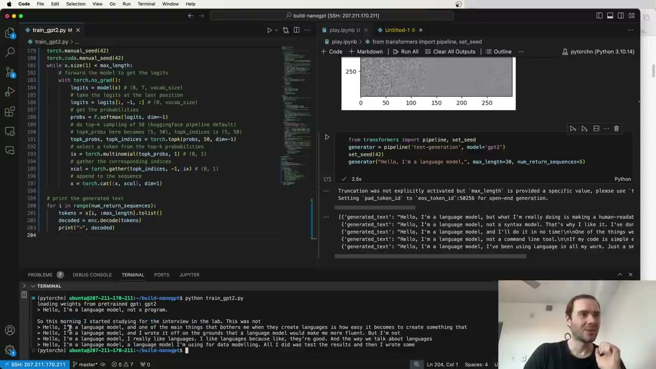 40:19
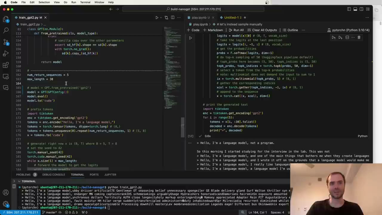 43:12
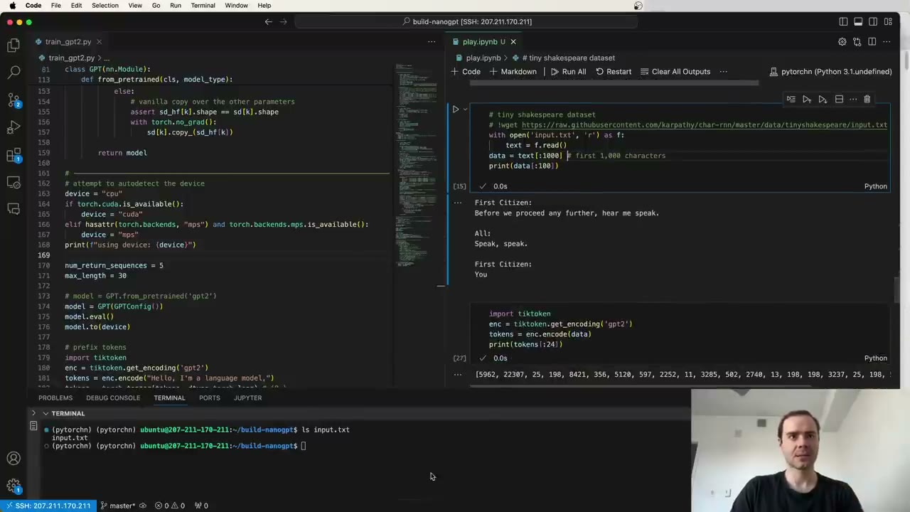 46:46
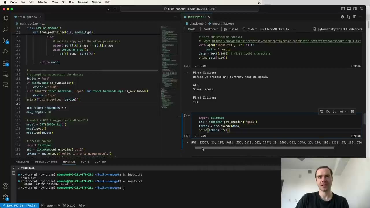 47:37
 50:59
 54:04
 55:10
 57:29
 1:01:25
 1:02:52
 1:06:05
 1:07:42
 1:08:33
 1:08:42
 1:10:37
 1:12:30
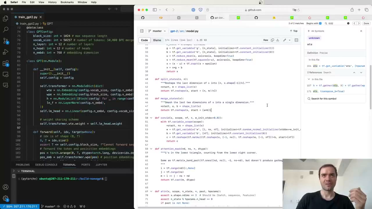 1:14:04
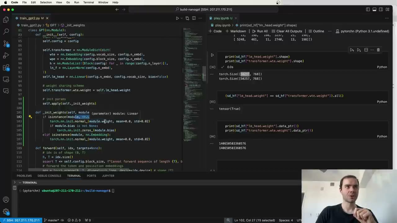 1:15:18
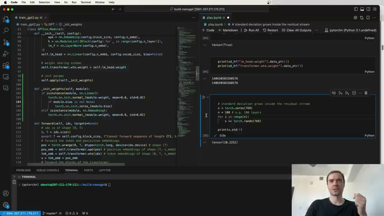 1:18:18
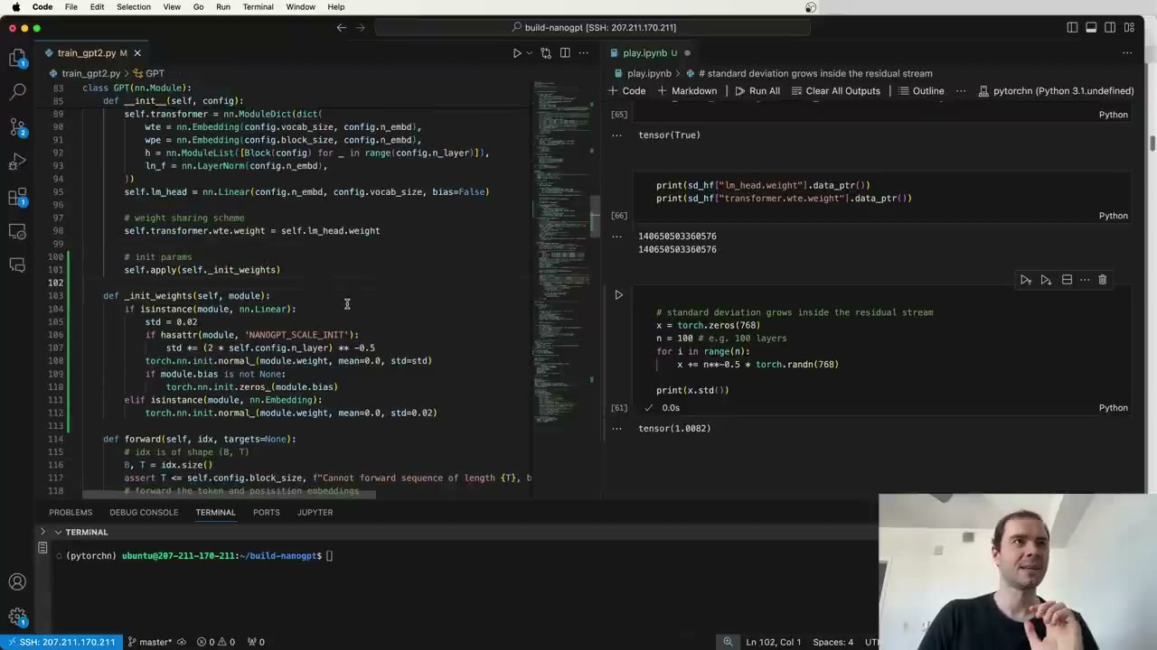 1:21:22
 1:22:56
 1:23:38
 1:28:24
 1:30:31
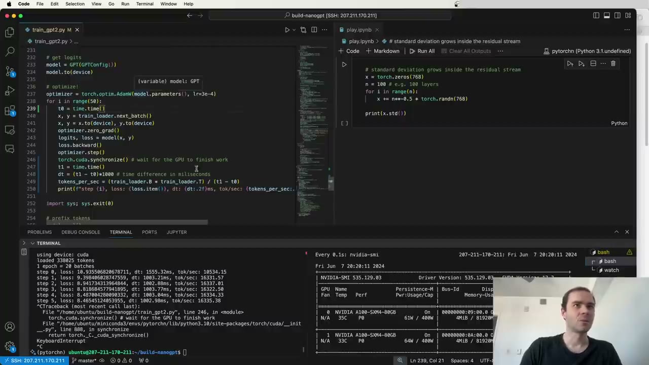 1:36:21
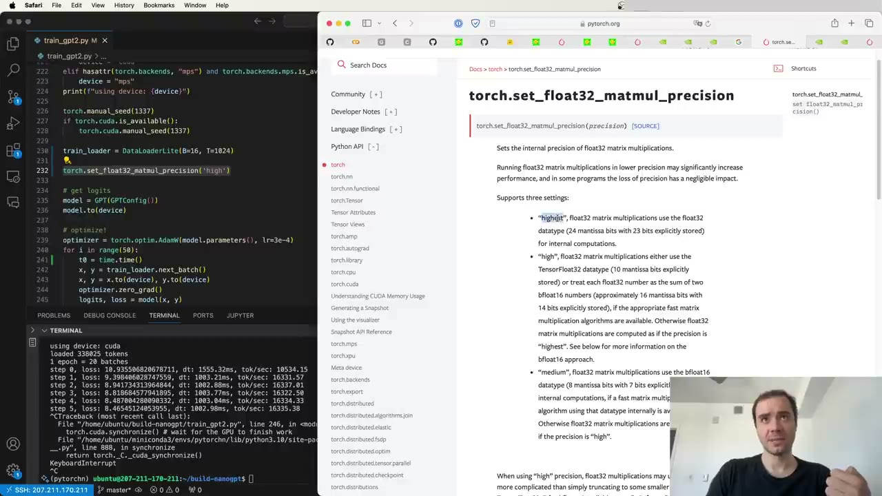 1:37:11
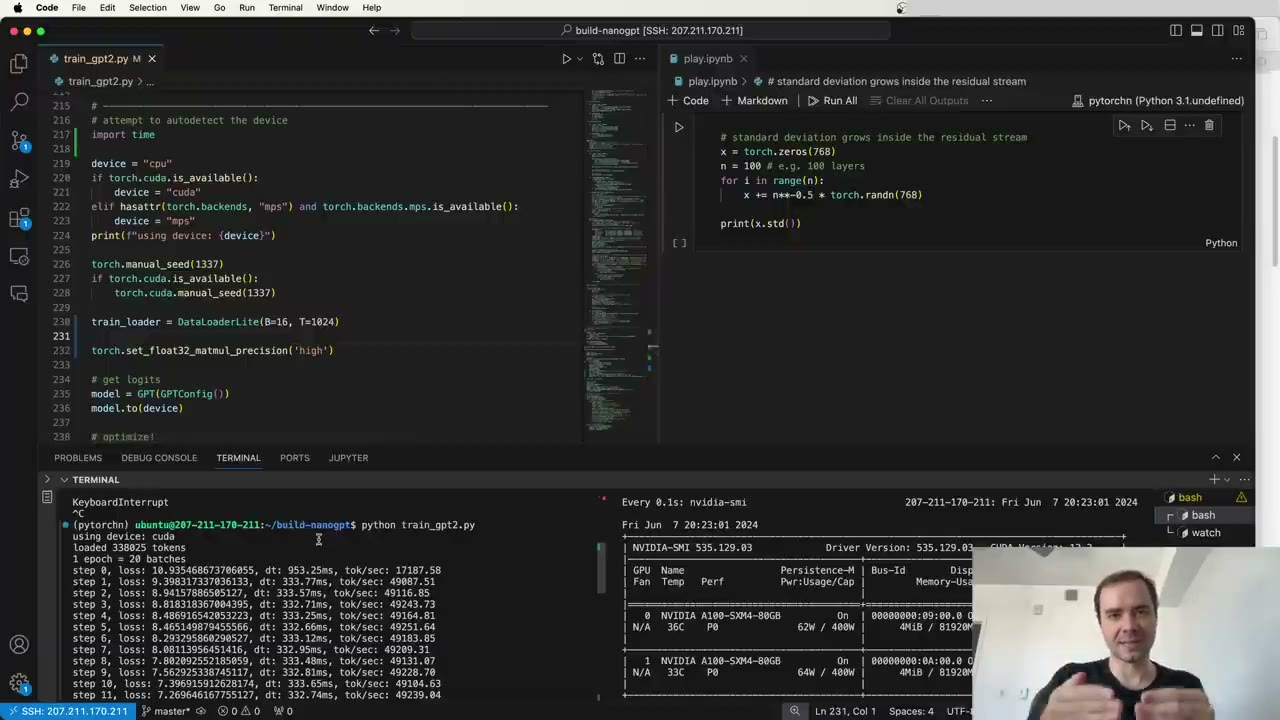 1:39:11
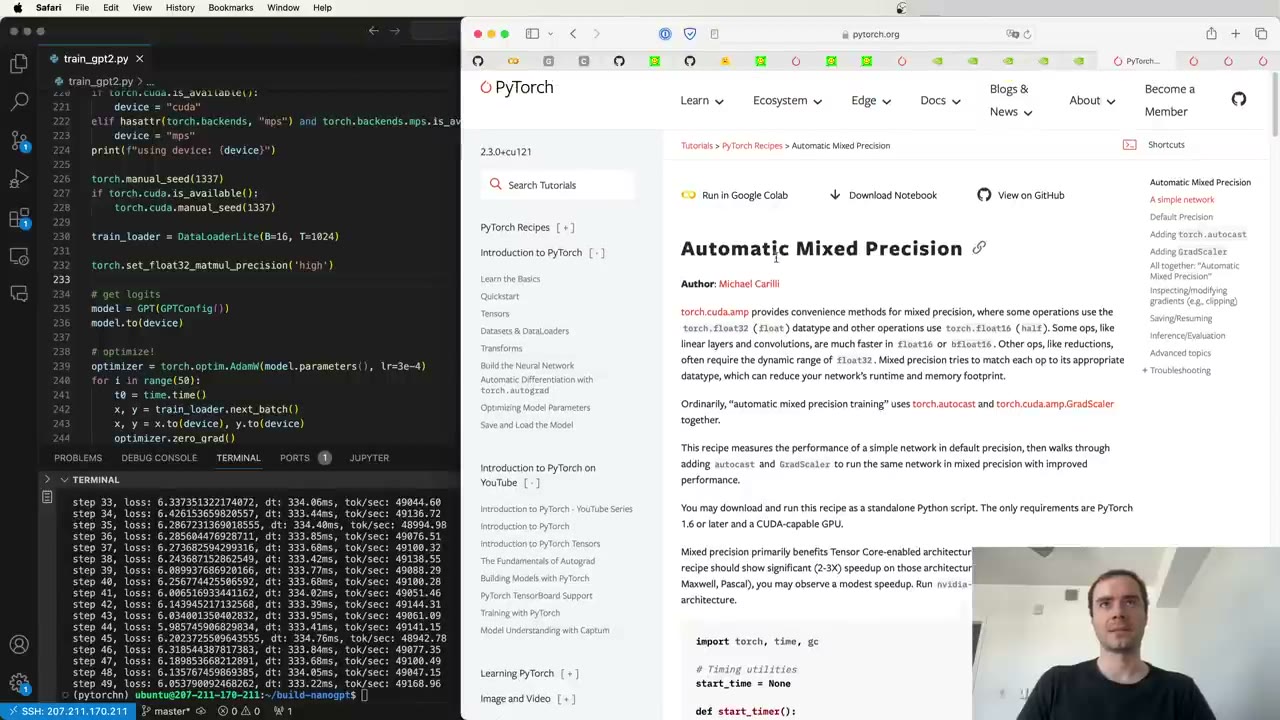 1:42:43
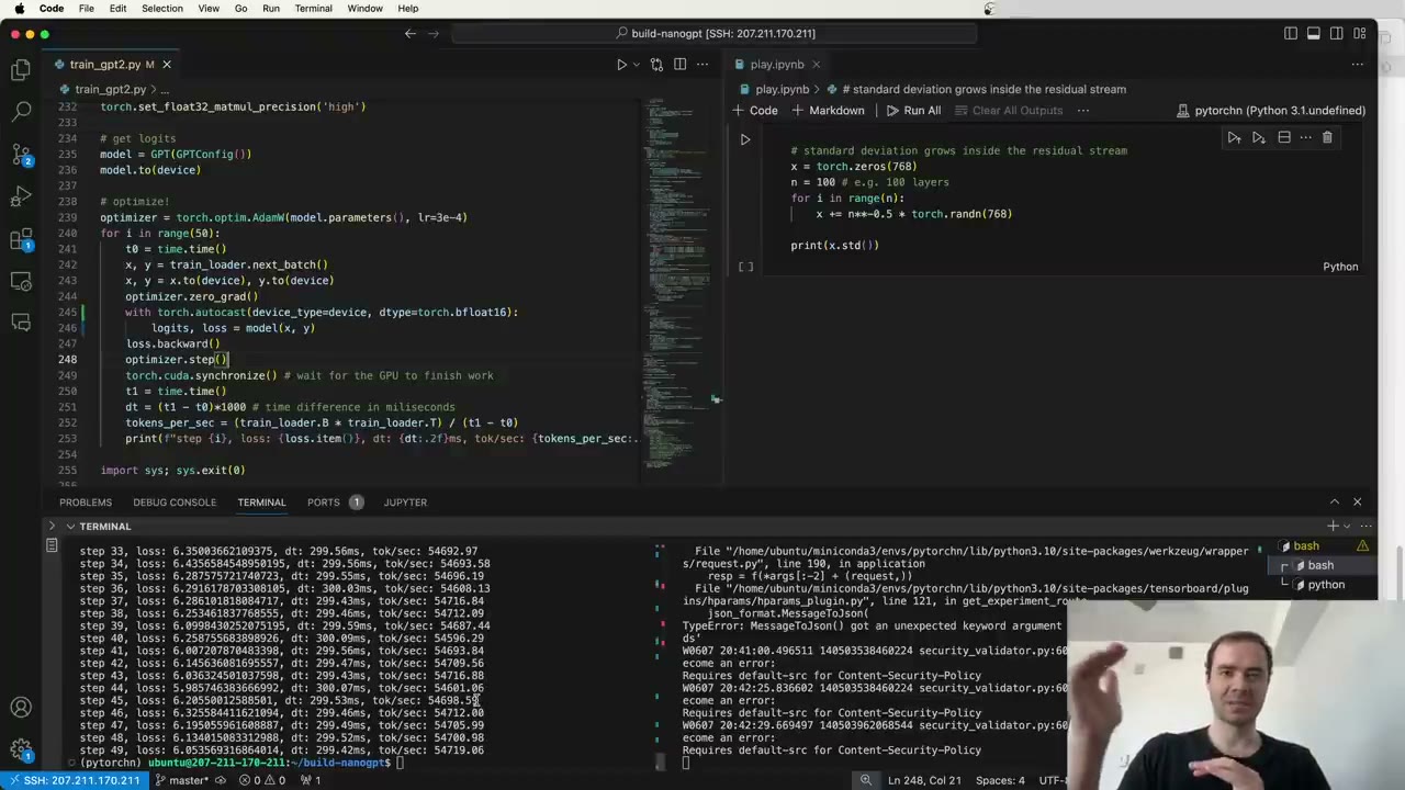 1:47:08
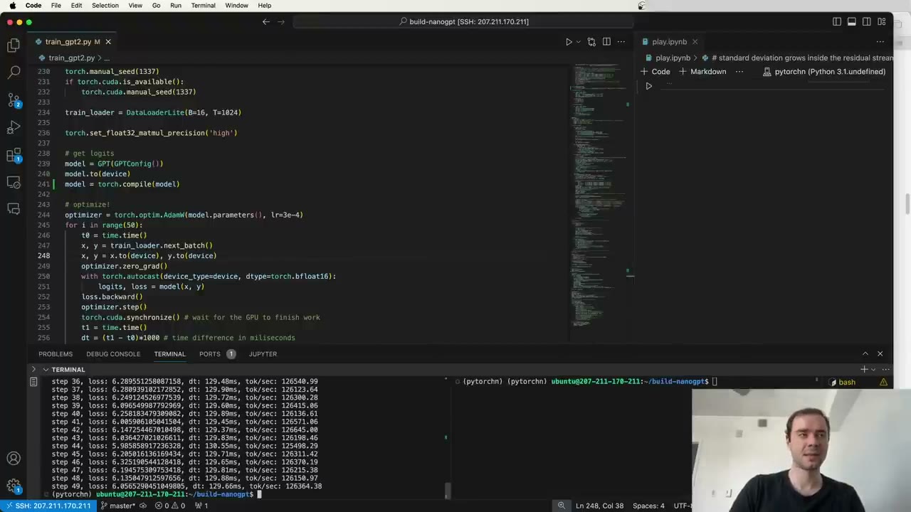 1:49:52
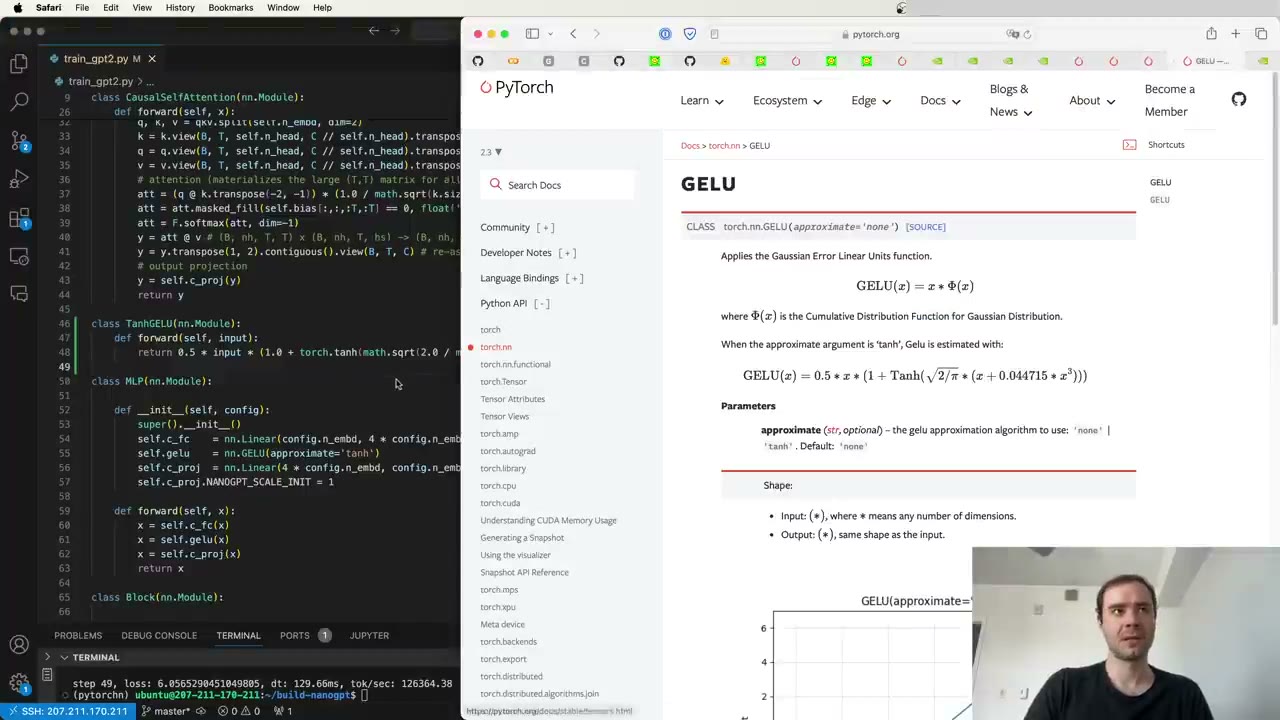 1:51:37
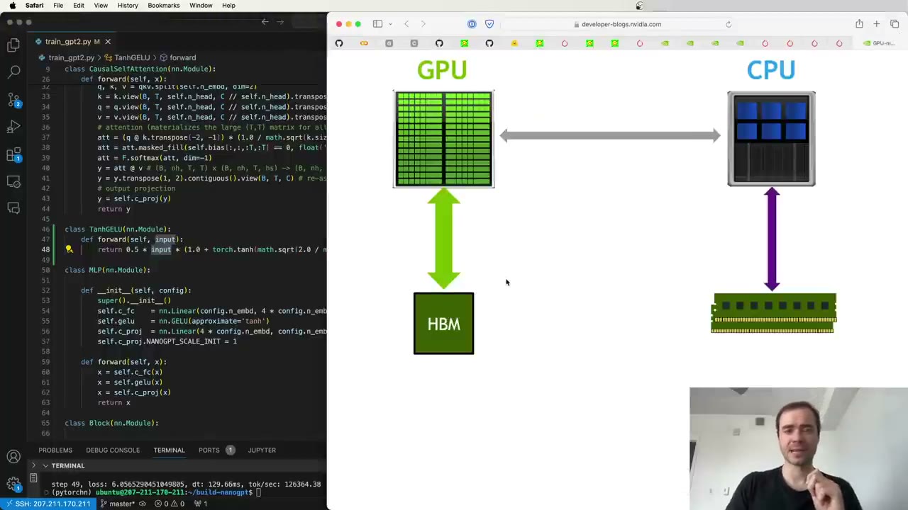 1:52:17
 1:56:02
 2:00:31
 2:00:57
 2:03:42
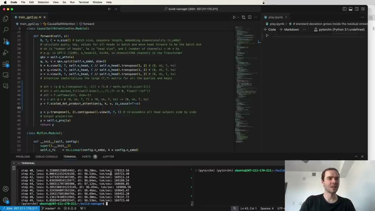 2:06:34
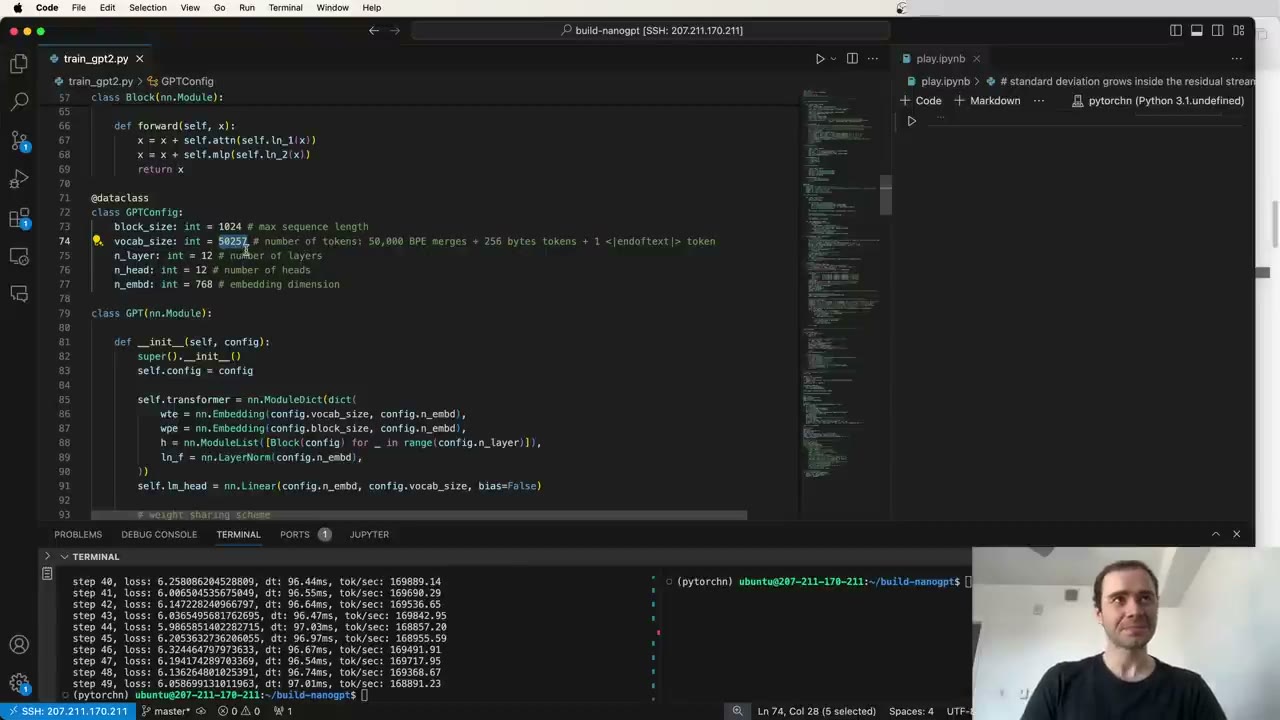 2:08:35
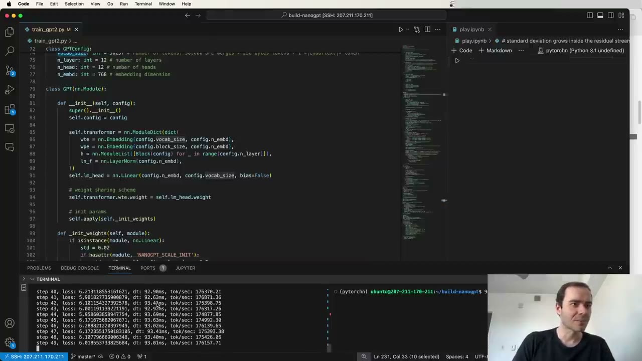 2:11:11
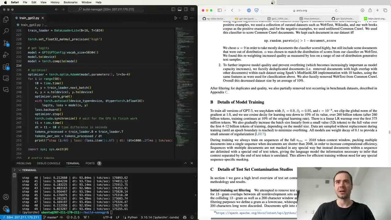 2:16:51
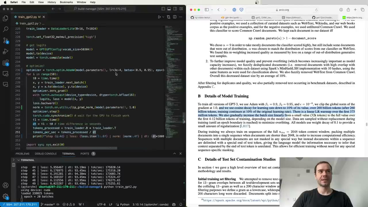 2:19:51
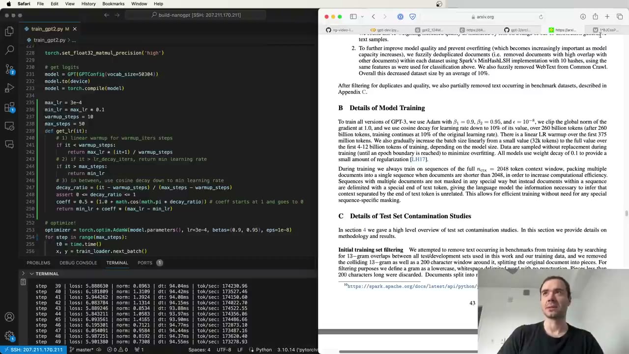 2:21:15
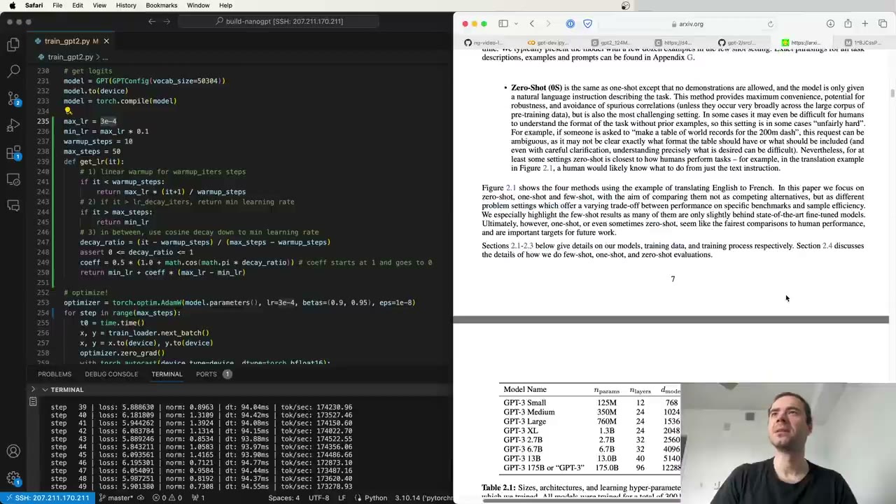 2:23:29
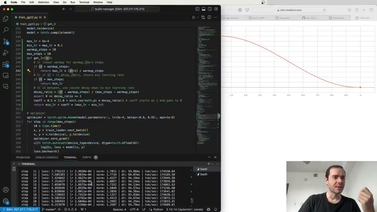 2:25:07
 2:29:50
 2:33:09
 2:36:07
 2:37:18
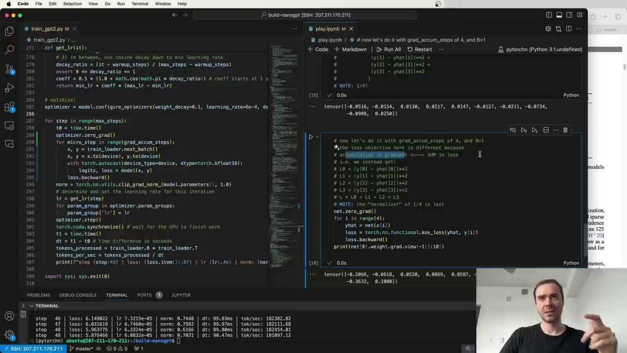 2:42:42
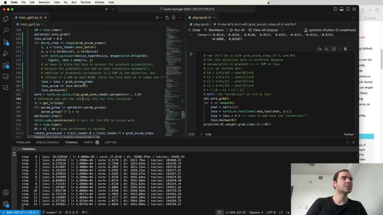 2:46:12
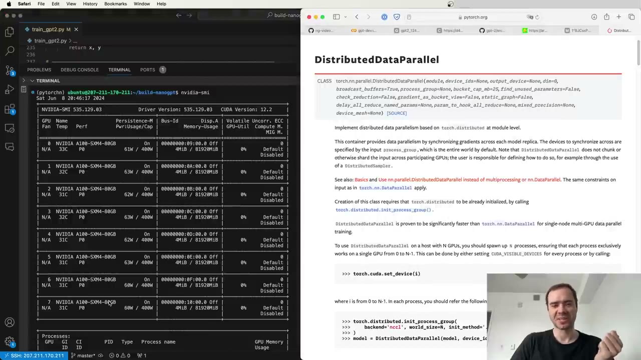 2:47:02
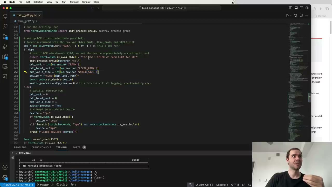 2:48:41
 2:56:27
 2:58:57
 3:00:37
 3:03:46
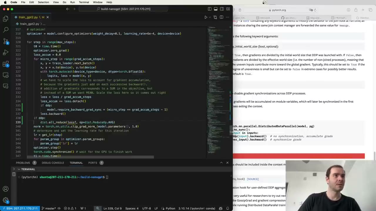 3:06:12
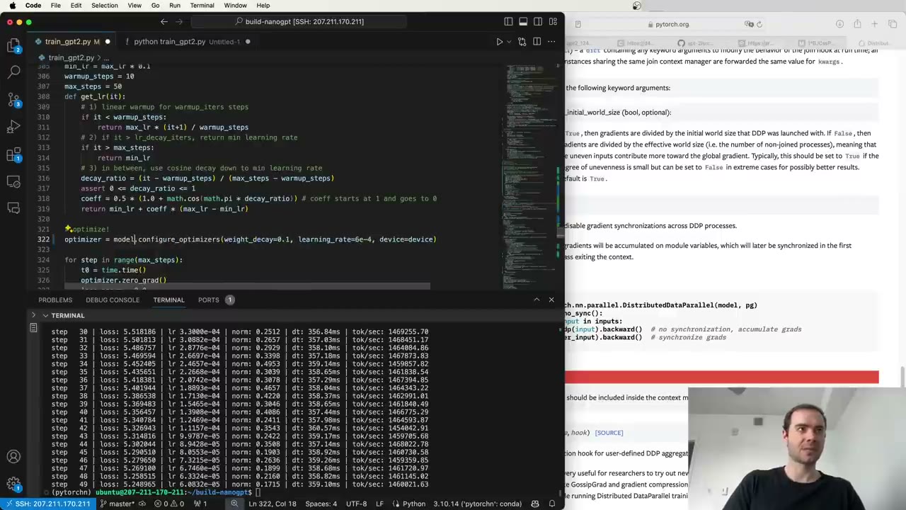 3:08:23
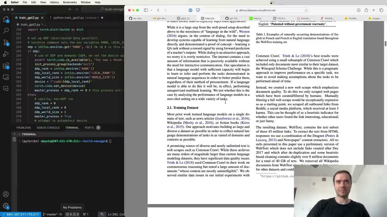 3:10:25
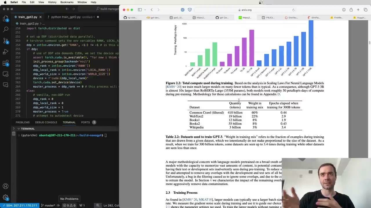 3:11:42
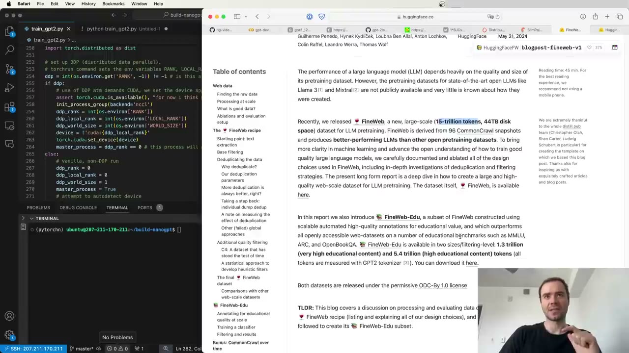 3:12:53
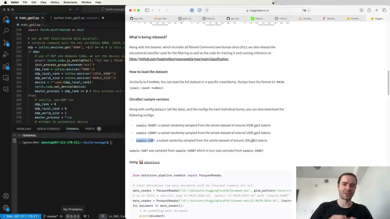 3:13:50
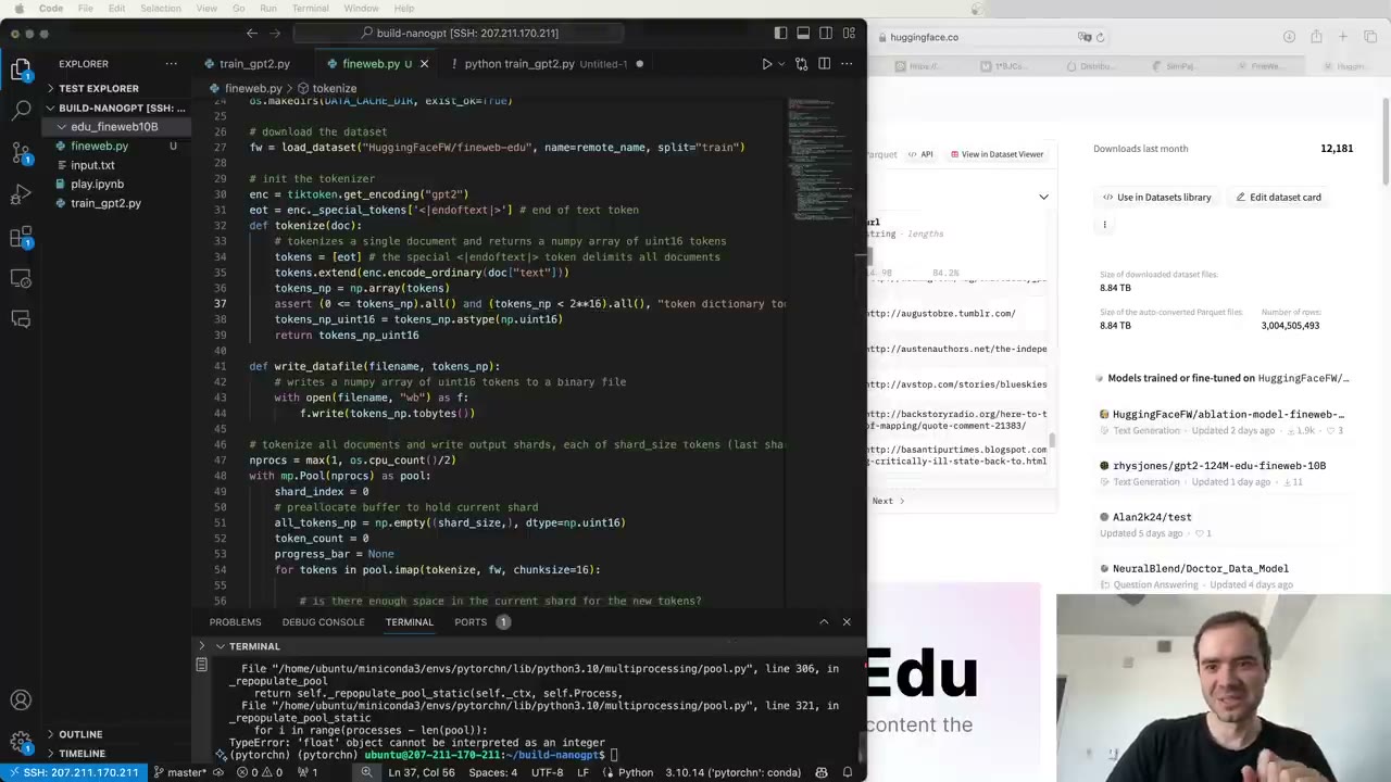 3:16:17
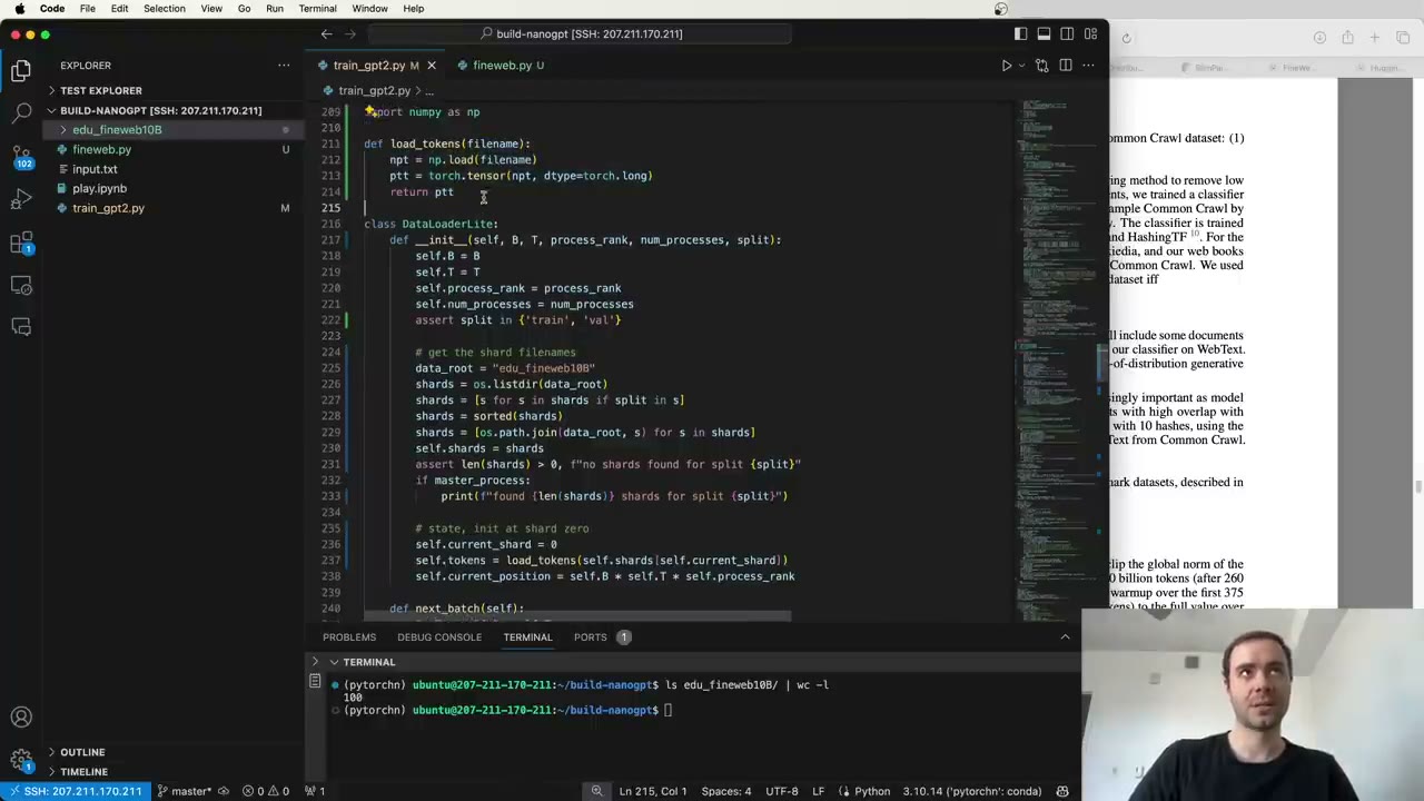 3:18:24
 3:20:10
 3:22:27
 3:23:42
 3:26:03
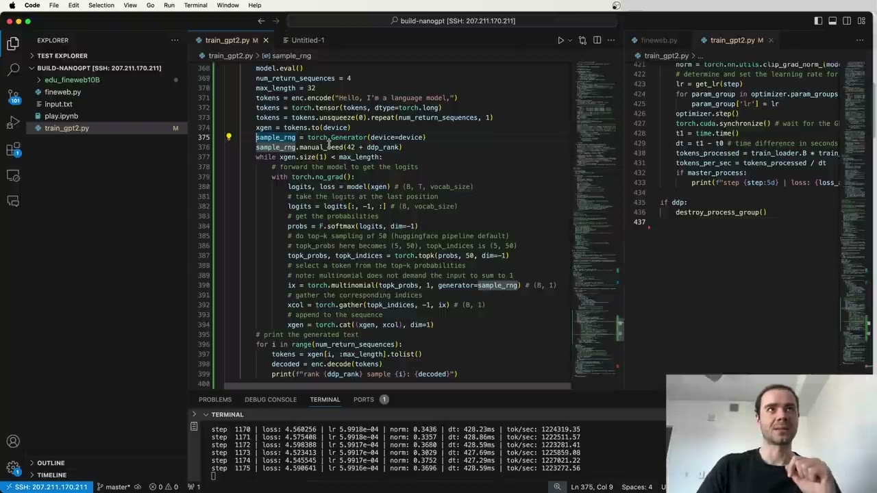 3:27:06
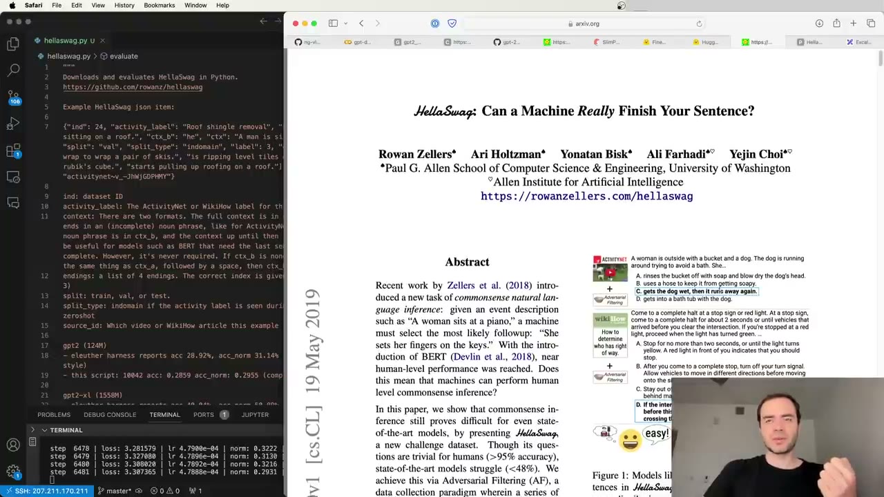 3:28:53
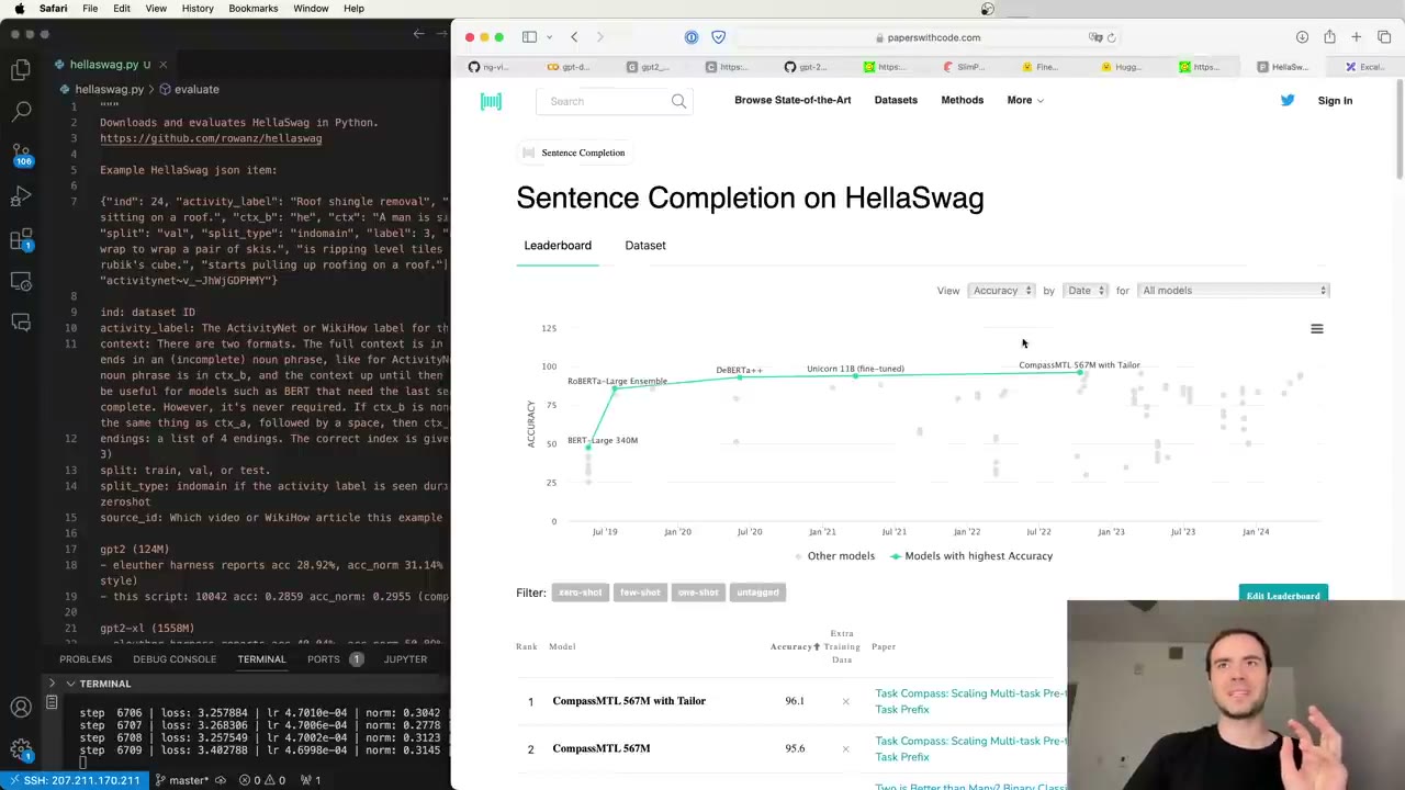 3:31:07
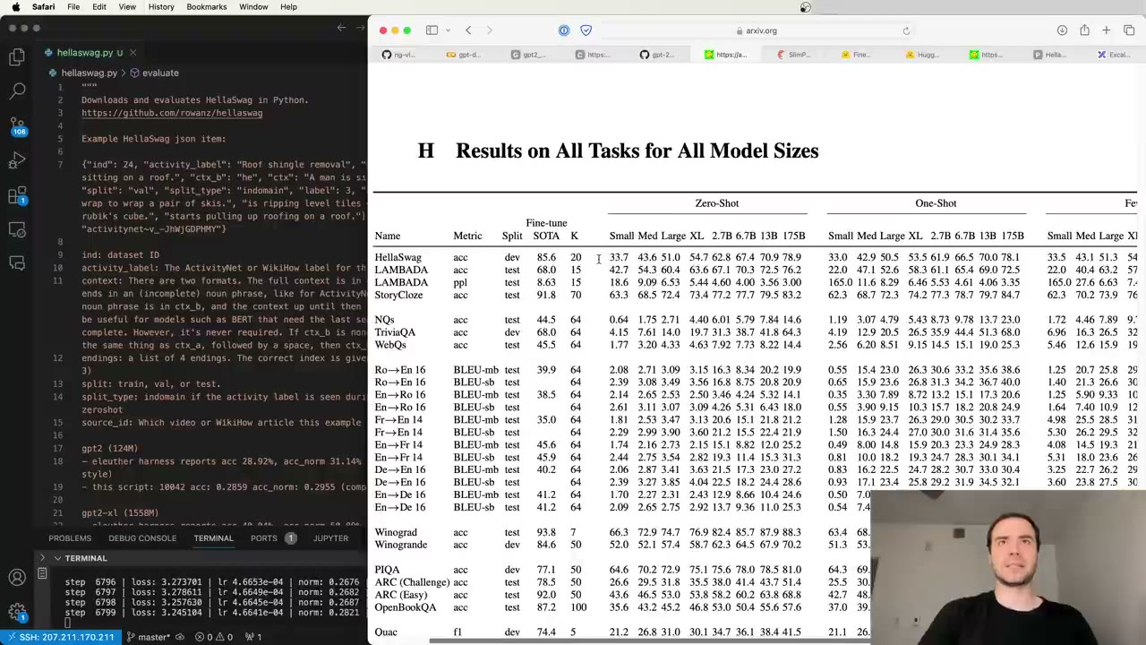 3:31:47
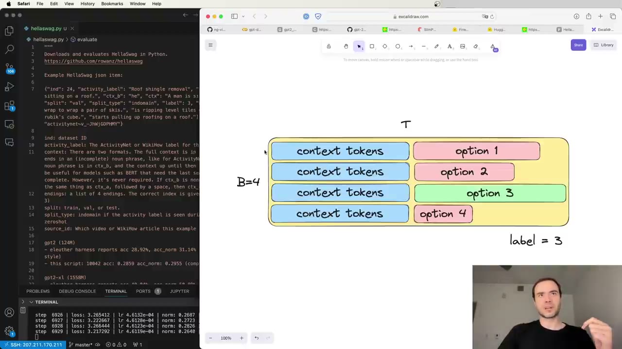 3:33:06
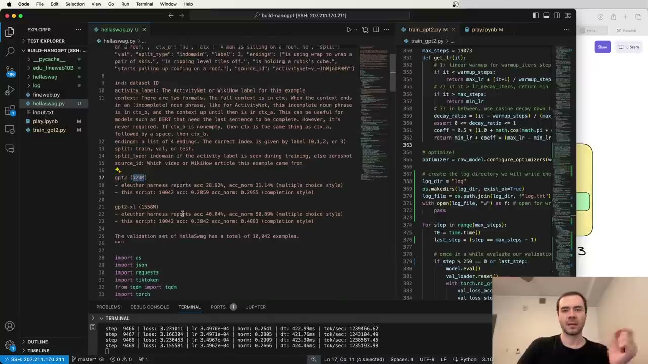 3:37:14
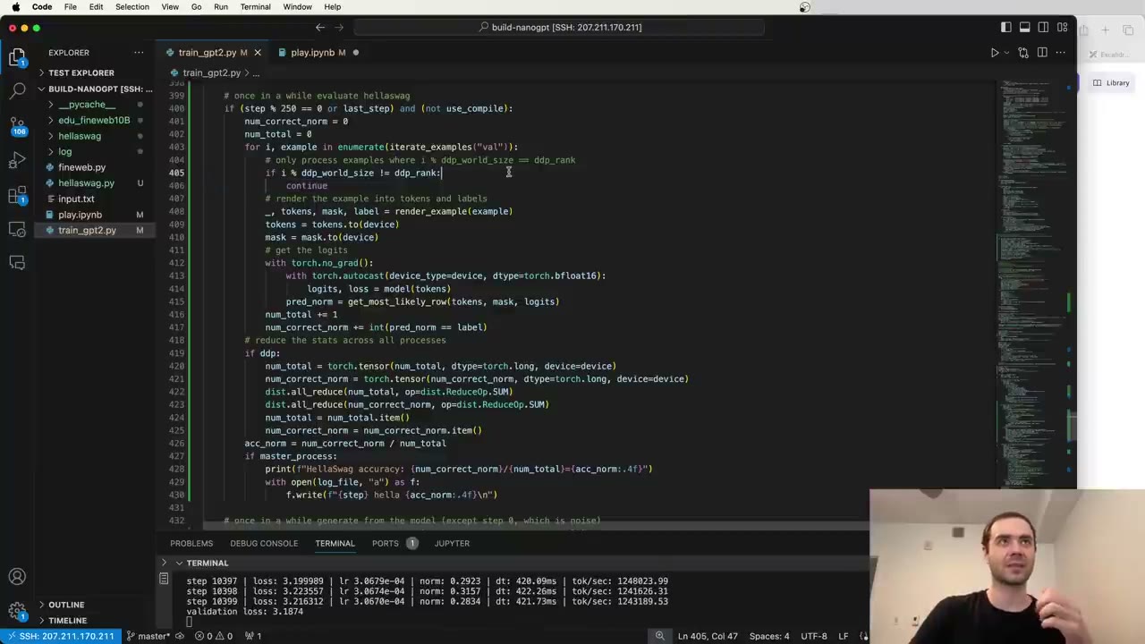 3:40:44
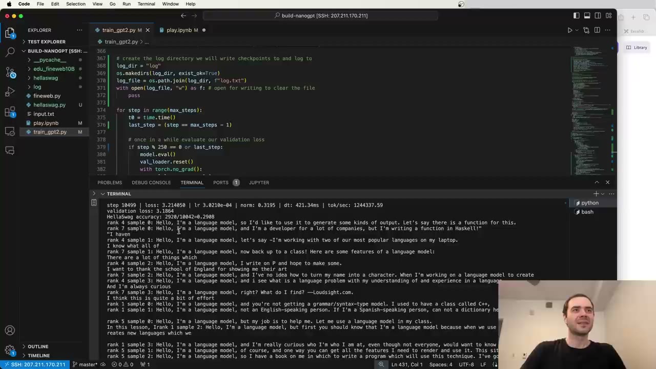 3:42:02
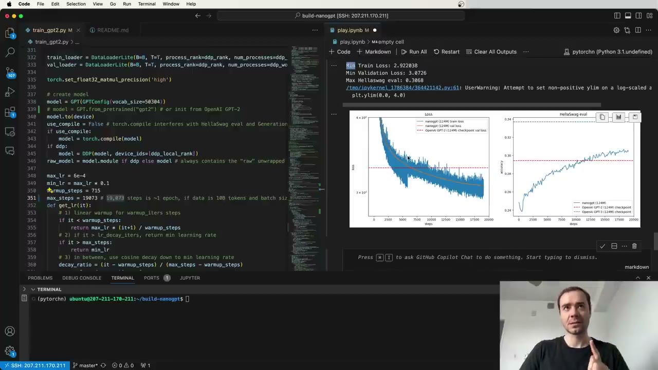 3:43:48
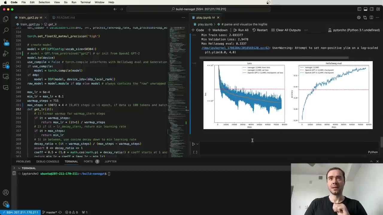 3:49:12
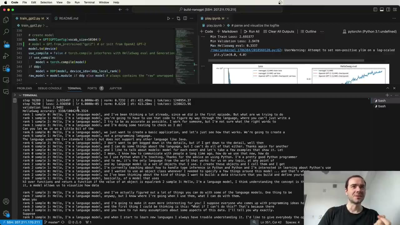 3:53:20
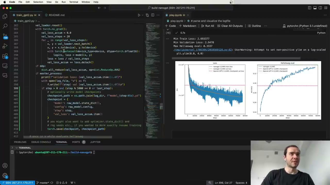 3:53:54
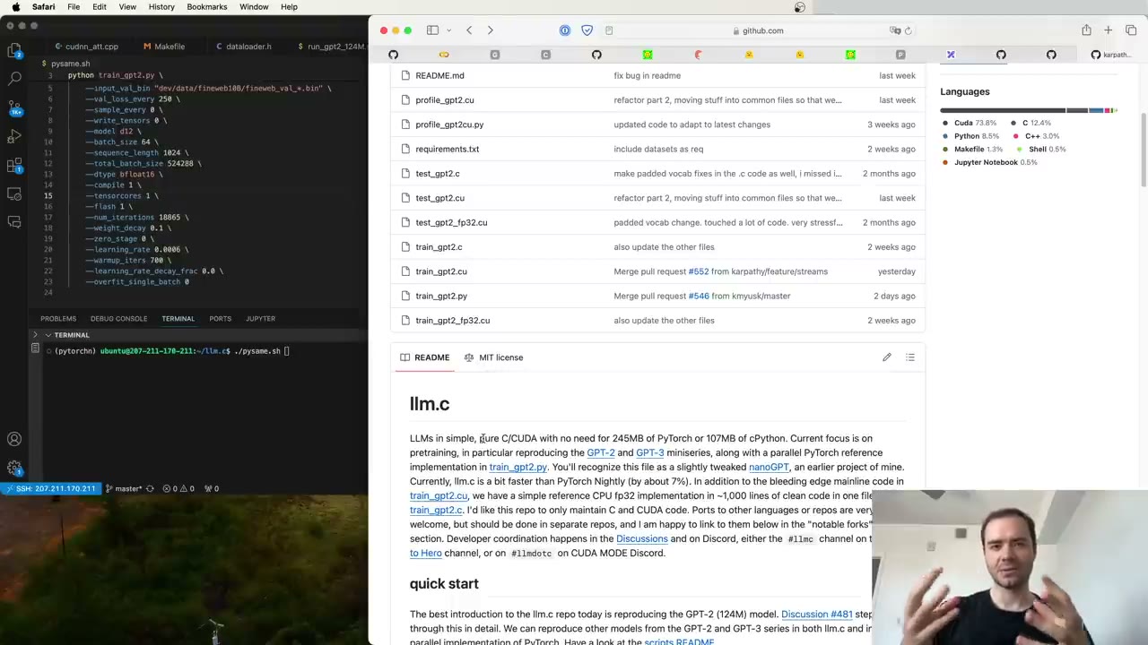 3:56:46
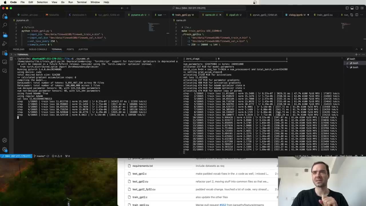 3:59:00
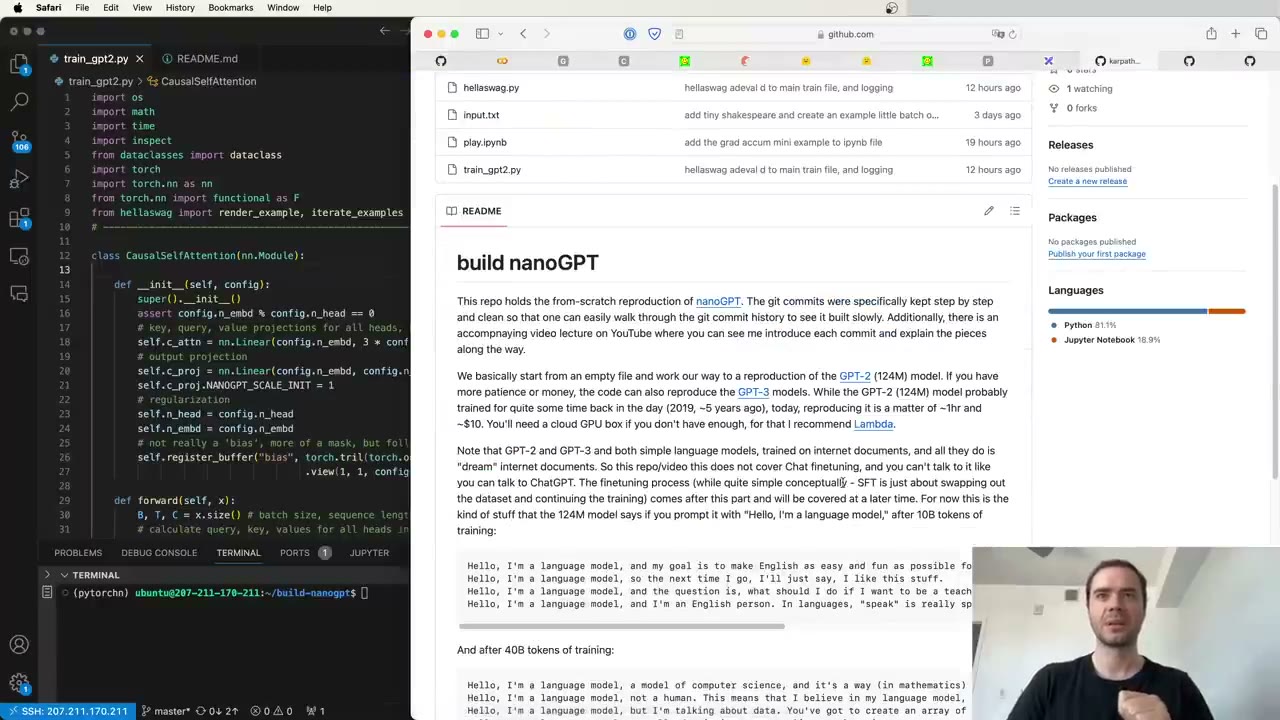 4:01:09
Watch the video (241 min)
Watch the original video on YouTube
Lecture 9 is the last video in Andrej Karpathy’s Neural Networks: Zero to Hero series and by far the longest, at just over four hours. It picks up two threads: the GPT model built from scratch in Lecture 7 and the GPT-2 tokenizer taken apart in Lecture 8. The goal is concrete: write GPT-2’s 124-million-parameter model yourself, check it against OpenAI’s released weights, then train it from random weights until it matches or beats the original. Roughly the first hour is the model and a basic training loop. The second hour is about speed, going from about 1,000 ms to 93 ms per step on one GPU. The third adds GPT-3’s optimizer recipe, gradient accumulation and eight-GPU training. The last hour covers the dataset, the evaluations, and the results of a two-hour and an overnight run. There is no next lecture; head back to the series index for the full course map.
Key takeaways
- Load the released weights before you train anything (12:34). If your own class can load OpenAI’s GPT-2 checkpoint and generate sensible text, you know the architecture is right, and training only has to find good weights.
- GPT-2 puts LayerNorm before each sublayer and keeps the residual stream clean (18:14). Gradients flow straight from the loss to the tokens through the additions, while attention (tokens exchange information) and the MLP (each token works alone) add refinements.
- The input embedding and the output layer share one matrix (1:12:57). Weight tying saves about 30% of the 124M parameters.
- Most of the speedup comes from moving less memory, not from doing fewer FLOPs (2:01:22). TF32, bfloat16, torch.compile, FlashAttention and a padded vocabulary together take one step from about 1,000 ms to 93 ms, roughly 11x (2:14:58).
- When the GPT-2 paper is vague, borrow GPT-3’s hyperparameters (2:16:34): AdamW with betas 0.9 and 0.95, gradient clipping at 1.0, cosine learning-rate decay with warmup, weight decay 0.1 and a 0.5M-token batch.
- Gradient accumulation needs the loss divided by the number of micro-steps (2:44:08). Without it, the gradients are too large by exactly that factor.
- Ten billion FineWeb-Edu tokens beat GPT-2 124M on HellaSwag (3:44:44). An overnight 40B-token run nearly reaches GPT-3 124M, though Karpathy lists several reasons to treat the comparison with care.
Chapter notes
0:02 – 3:36 The target: GPT-2 124M
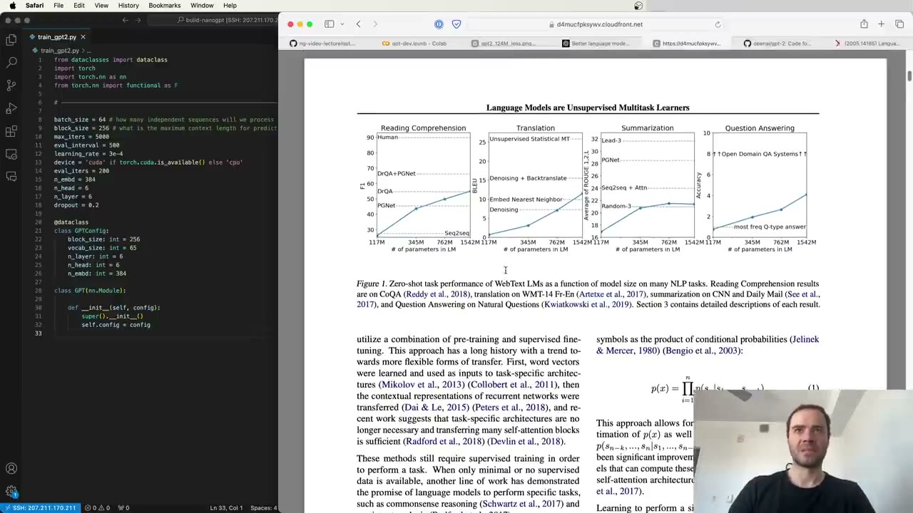
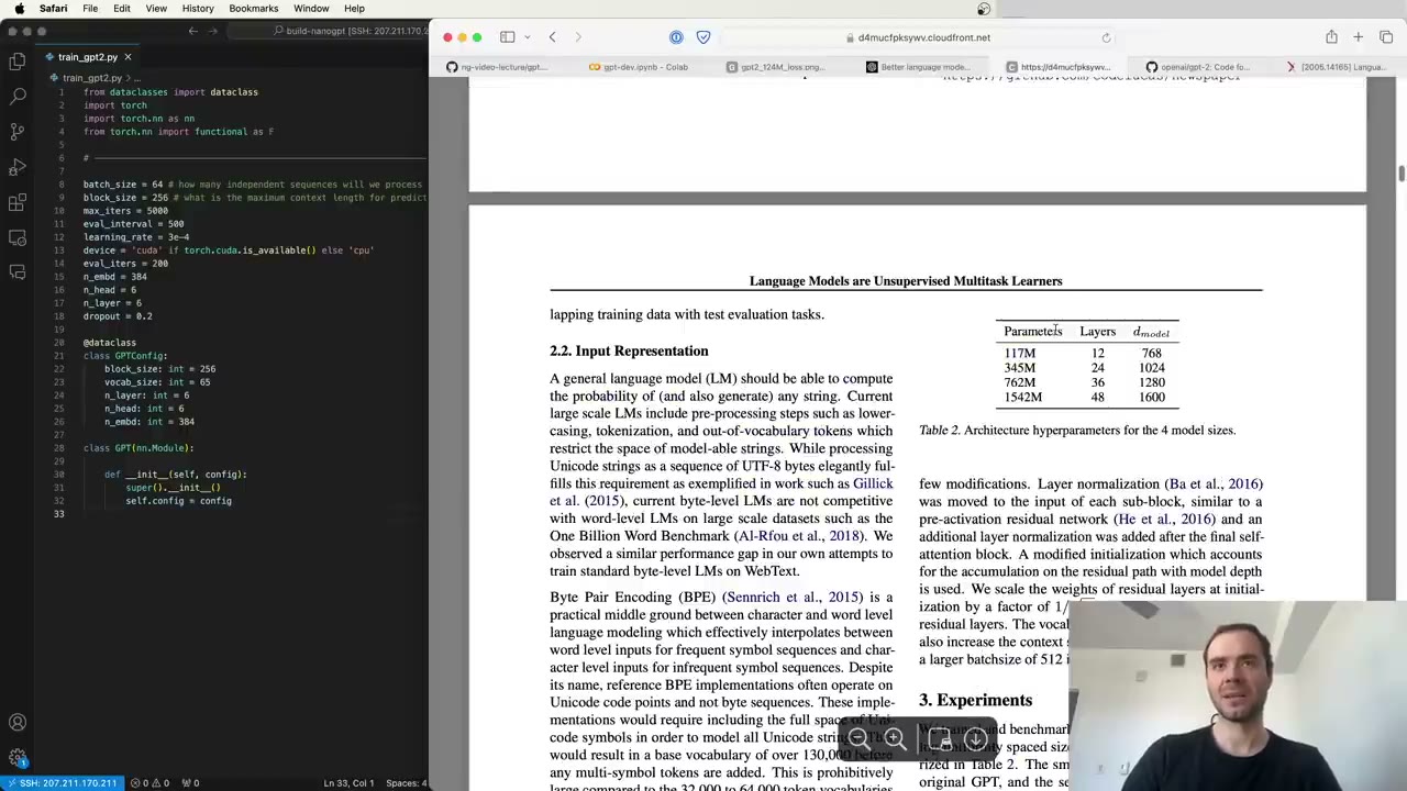
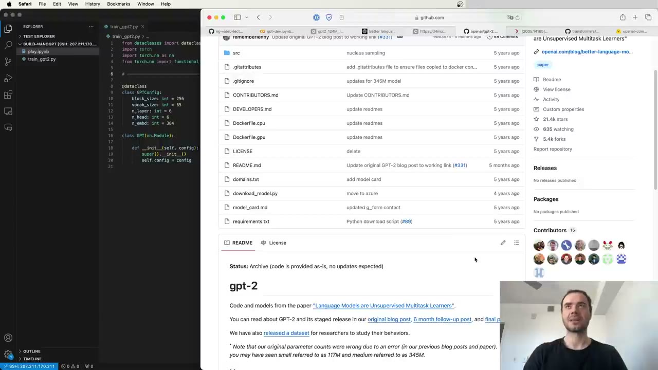
OpenAI released GPT-2 in 2019 with a blog post, a paper and code. Like most such releases it is a miniseries, four models of increasing size, so that downstream scores can be plotted against model size to show scaling (0:33). Karpathy names the sizes 124M to 1558M and notes that the parameter counts in the paper’s table are wrong, as the GPT-2 repo itself acknowledges (1:03). The target is the smallest: 12 layers and 768 channels (1:33). He assumes you have seen the earlier “Let’s build GPT” lecture.
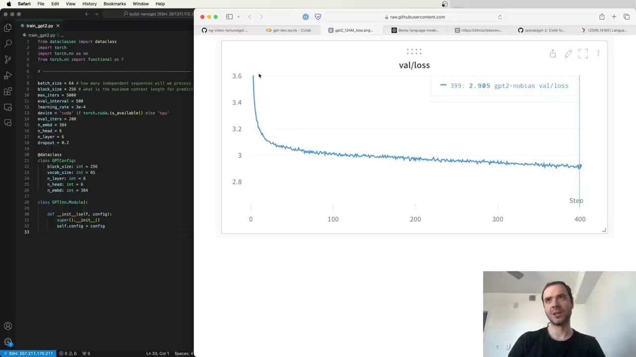
The finish line is a validation-loss curve that falls below the released GPT-2 124M (2:04). What was a serious effort five years ago is now, he says, about an hour on a rented machine for about 10 dollars (2:35). OpenAI released the weights, but the GPT-2 paper is thin on training details, so the video also leans on the GPT-3 paper, whose architecture is close and whose hyperparameters are spelled out (3:06).
Our note: the GPT-2 paper’s table lists 117M, 345M, 762M and 1542M parameters. The 124M and 1558M figures Karpathy uses are the corrected counts.
3:36 – 13:34 Taking the released model for a spin
Before writing any code, Karpathy loads the target model. OpenAI’s original code is TensorFlow, so he uses Hugging Face Transformers instead, which has already converted the weights to PyTorch (4:09). One naming quirk: the model id gpt2 is the 124M model, and the 1.5B model is gpt2-xl (5:15).
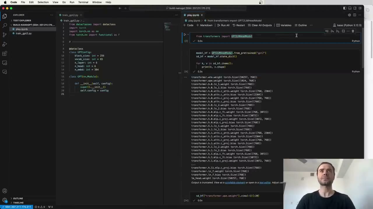
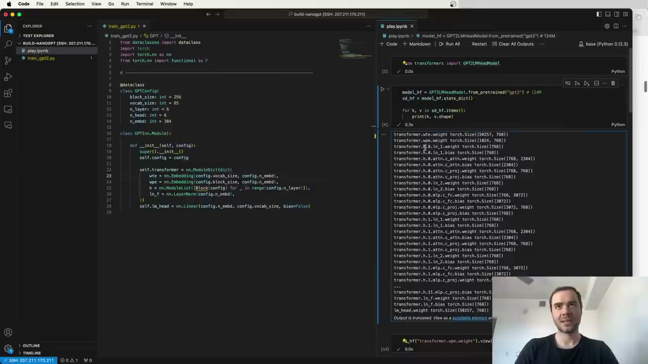
He prints the state dict, which is just the raw tensors and their names. The token embedding table is 50257 × 768, one 768-number vector for each token in the GPT-2 vocabulary (6:17). The position embedding table is 1024 × 768, because GPT-2 can look back over at most 1,024 positions (6:49).
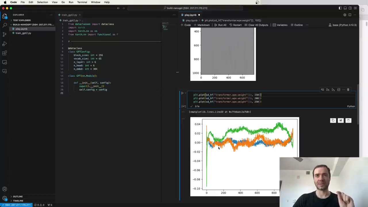
Plotting the position embeddings shows clear structure (7:56). Individual channels respond to particular ranges of position, and the curves look roughly like sines and cosines. That is notable because these vectors start as random noise and are learned. The original Transformer paper fixed them to sinusoids; GPT-2 trains them, and something sinusoid-like falls out of the optimization anyway (10:01). He reads the jaggedness of the curves as a sign that the model was somewhat undertrained (9:30).
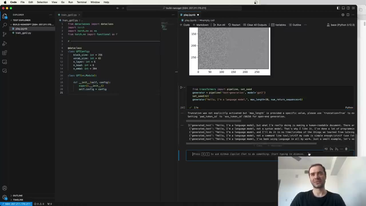
Sampling through the Hugging Face pipeline with the prefix “Hello, I’m a language model,” gives five coherent completions (11:33). The plan from here (12:34): write a short GPT-2 class of our own, load these weights into it to prove it is the same model family, then throw the weights away and train from scratch (13:04).
13:34 – 28:07 Writing GPT-2 as a PyTorch module
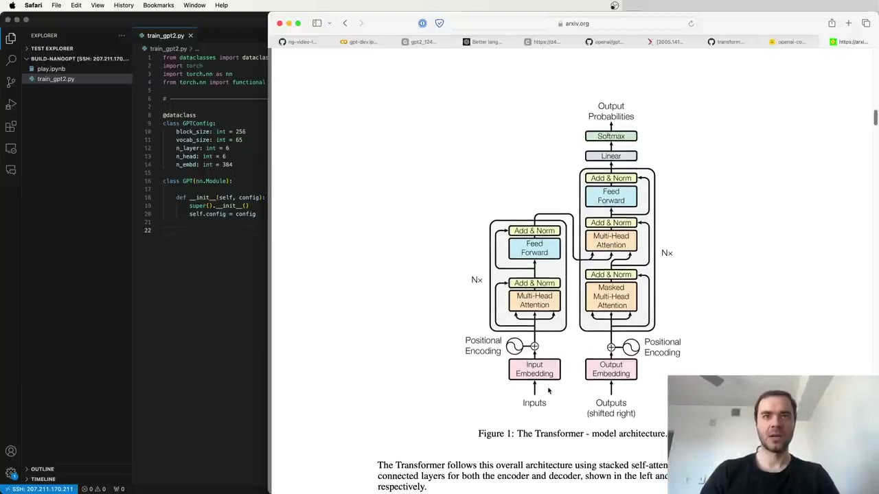
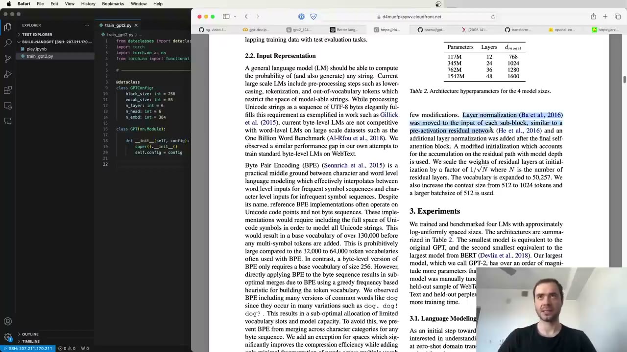
GPT-2 is a decoder-only Transformer. Compared with the “Attention Is All You Need” diagram, the encoder and the cross-attention that reads from it are gone (13:34). Two more changes come from the GPT-2 paper: each LayerNorm moves to the input of its sublayer, and an extra LayerNorm is added before the final classifier (14:05).
The skeleton deliberately copies Hugging Face’s names, so loading weights becomes a matter of matching keys (14:38). A ModuleDict called transformer holds wte (token embeddings), wpe (position embeddings), h (a ModuleList of 12 blocks) and ln_f (the final LayerNorm). Then lm_head projects from 768 channels to the 50,257-token vocabulary, without a bias (16:42).
The block is where the pre-norm change shows (17:43). In the original Transformer, normalization sits inside the residual path. Karpathy explains why you want the residual stream clean instead (18:14): addition passes its incoming gradient to both branches unchanged (the micrograd lesson), so a clean stream gives the gradient a highway from the loss straight down to the token embeddings, and the blocks contribute their part on top of it.
His framing of what the block does (19:47): attention is where the 1,024 tokens communicate, a weighted sum or pooling across positions, while the MLP processes each token on its own. So a Transformer is a repeated map-reduce, with attention as the reduce and the MLP as the map (20:18).
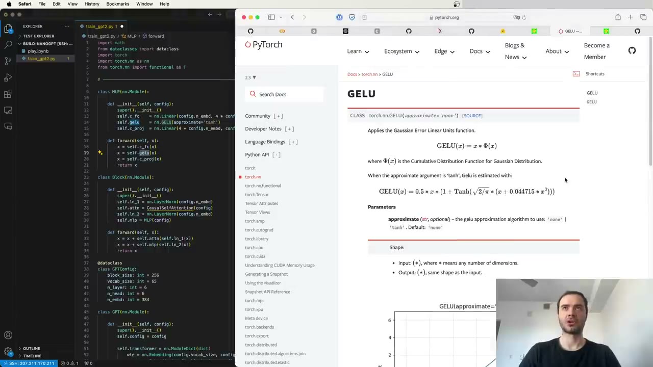
The MLP is two linear layers around a GELU (20:48). GPT-2 used the tanh approximation of GELU, a historical leftover: according to Dan Hendrycks’s GitHub comment, the exact version needed an erf function that was slow in TensorFlow at the time (21:51). Karpathy keeps the approximation only to stay faithful. The reason to prefer GELU over ReLU is that it never has a perfectly flat region, so no neuron gets stuck with zero gradient (22:55). Newer models such as Llama 3 have moved on to SwiGLU and similar variants (23:25).
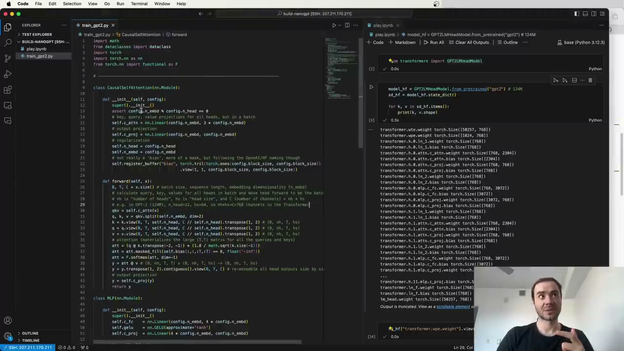
Attention is the same algorithm as in Lecture 7, but written for speed (23:57). Instead of separate head modules whose outputs are concatenated, one linear layer produces queries, keys and values for all heads at once, and the heads are folded into a batch dimension so PyTorch processes them in parallel (26:03). The steps are unchanged: query-key dot products, the causal mask so tokens only see the past, a softmax, and a weighted sum of the values. The finished model is under 100 lines, against about 2,000 in the Hugging Face file (27:36).
28:07 – 41:44 Loading the weights and generating text
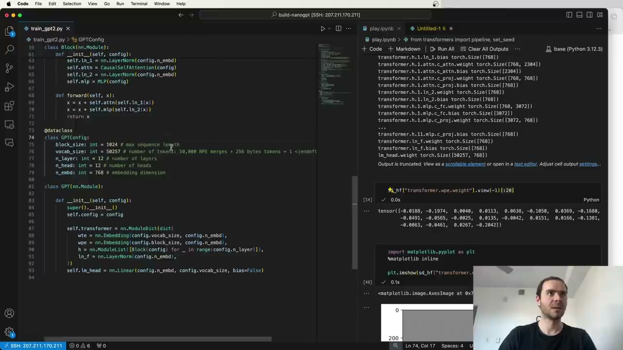
The config matches GPT-2 124M (28:07): block_size 1024 and vocab_size 50257, which is 50,000 BPE merges plus 256 byte tokens plus one end-of-text token. Then 12 layers, 12 heads and 768 embedding dimensions (28:38).
A from_pretrained class method builds the model and copies the tensors over key by key (29:08). Two wrinkles. The attn.bias entries are buffers holding the causal mask, not parameters, so they are skipped. And because the weights came from TensorFlow, a hard-coded list of weight matrices has to be transposed (29:42).
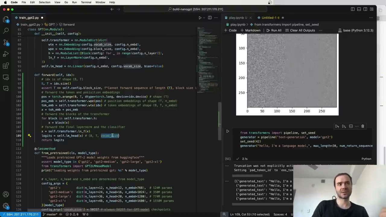
The forward pass takes token indices of shape (B, T) (30:44), builds the position indices on the same device as the input (31:46), adds the position embeddings (broadcast across the batch) to the token embeddings, runs the blocks and the final LayerNorm, and returns logits of shape (B, T, vocab_size) (32:46). Each position’s logits are a softmax away from a distribution over the next token.
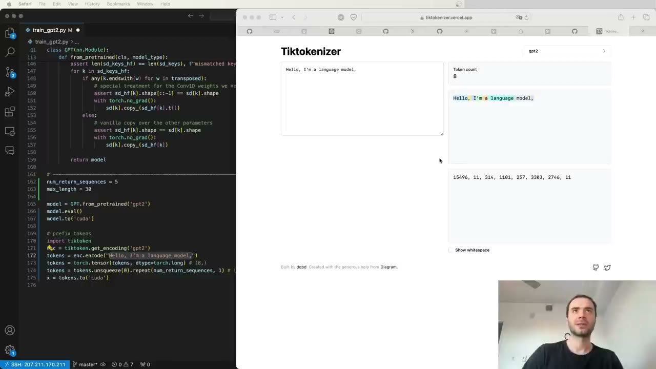
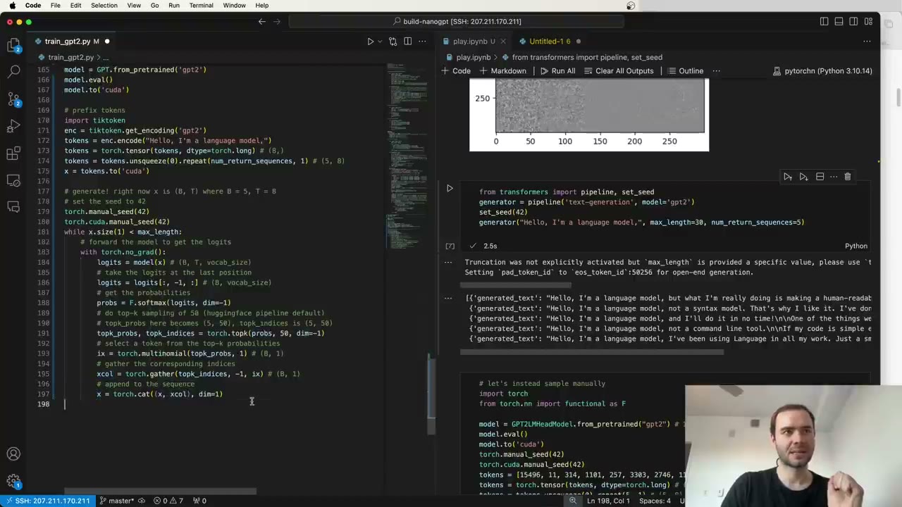
Generation mirrors the Hugging Face demo (33:48). The model goes into eval() mode, which may do nothing here since there is no dropout or BatchNorm, and moves to the GPU. The prefix is encoded with OpenAI’s tiktoken into eight tokens and repeated into five rows (35:20). Each loop iteration, inside torch.no_grad(), takes the logits at the last position only, applies softmax, keeps the top 50 tokens (Hugging Face’s default), renormalizes and samples one token per row (37:54). Top-k stops the model from wandering into very rare tokens (38:56).
The output is coherent but not identical to the pipeline’s (40:11). Karpathy could not find which pipeline setting causes the difference. Running the Hugging Face model with his own sampling code does reproduce his results, so the weights are loaded correctly (40:43).
41:44 – 52:38 From random weights to a first batch
Swapping in a randomly initialized model is one line, GPT(GPTConfig()), because PyTorch layers come with default initializations (42:15). The samples are now random token soup.
For readers without a GPU, he adds device auto-detection (43:16): try CUDA, then MPS (the Apple Silicon GPU backend), then fall back to CPU. Because the position indices are created on the input’s device, the same code runs anywhere. On the CPU the sampling demo took about six seconds (44:49), though the multi-GPU parts at the end are out of reach.
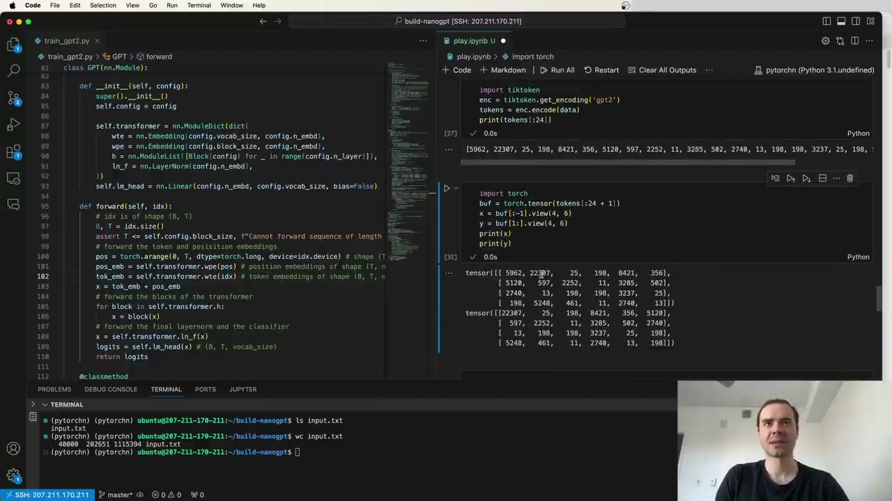
The debugging dataset is Tiny Shakespeare (45:51): about 40,000 lines, 200,000 words and a million ASCII characters, which at GPT-2’s roughly 3:1 compression comes to about 300,000 tokens (46:22). Token 198 is the newline (47:23).
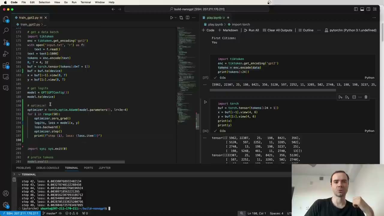
His favorite batching trick (48:25): take a flat run of B·T + 1 tokens. Everything except the last token, reshaped with .view(B, T), is the input; everything except the first, reshaped the same way, is the target (50:30). The extra token is what gives the final position in the batch its label, and each target sits at the same index as the input it belongs to.
52:38 – 1:06:18 Loss, AdamW and a tiny data loader
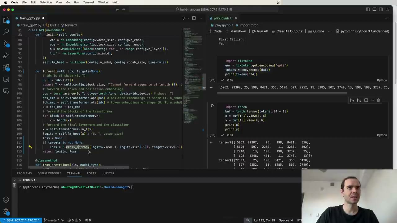
forward now accepts optional targets and returns the loss as well as the logits (52:38). F.cross_entropy will not take a (B, T, vocab) tensor, so logits are flattened to (B·T, vocab) and targets to (B·T) (54:17).
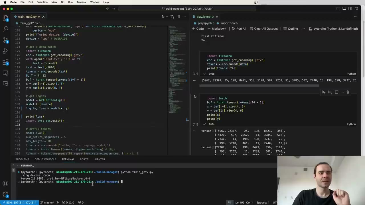
The first loss is a sanity check (55:18). A well-initialized network should spread probability roughly evenly over the vocabulary, giving a loss near −ln(1/50257) ≈ 10.82. He sees about 11, so the network is not confidently wrong at the start (55:49).
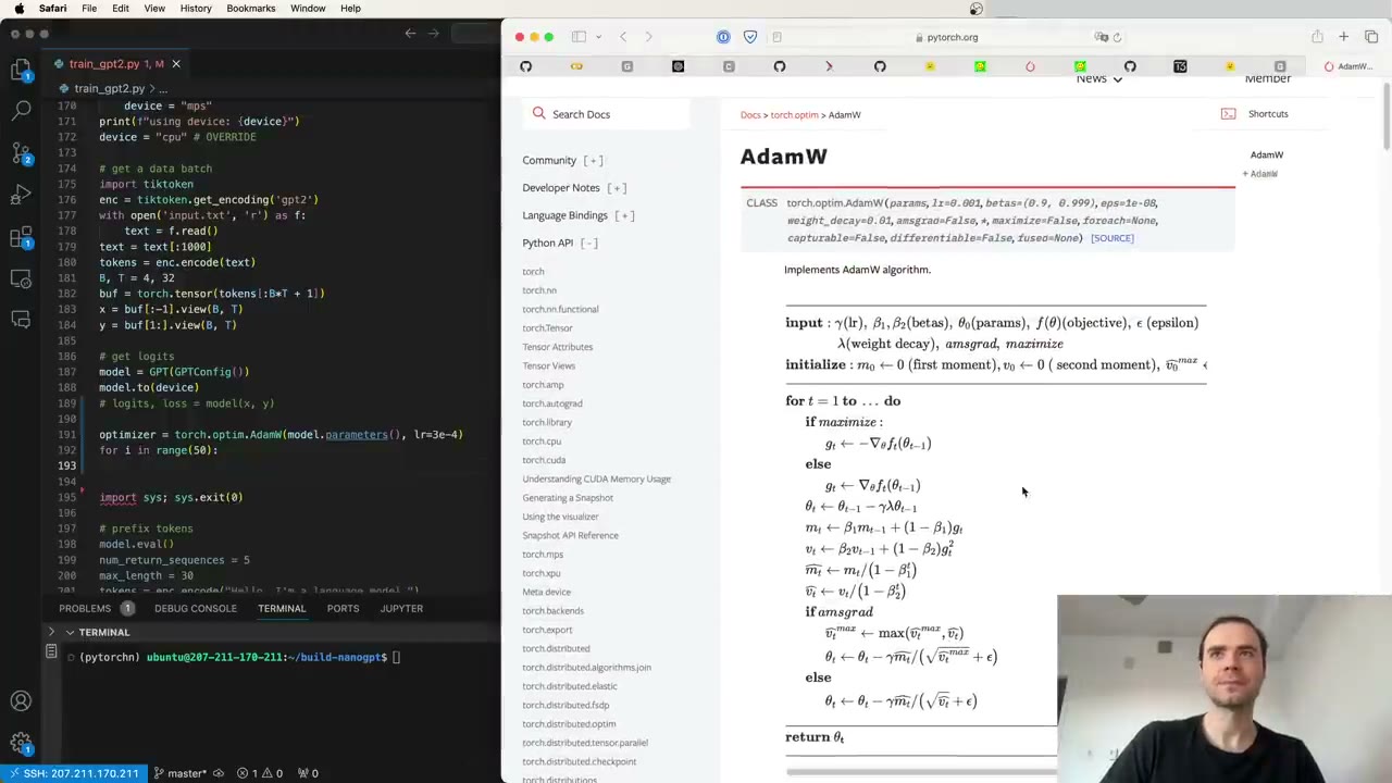
The optimizer is AdamW rather than plain SGD (56:51). He calls it a bug fix of Adam and treats it as a black box: it keeps two running buffers per parameter, m and v, similar to momentum and RMSProp, and that per-element normalization speeds up language models in particular (57:22). Two reminders in the loop: zero the gradients first, because backward() always adds to them (58:30), and loss.item() copies the single number from the GPU back to the CPU (59:00).
A live bug: the token buffer stayed on the CPU, because for tensors .to(device) returns a new tensor instead of changing the old one, unlike for modules (1:00:06). Once fixed, 50 steps on a single repeated batch at learning rate 3e-4 drive the loss toward zero (1:01:08). Overfitting one batch is the standard check that the model can learn at all.
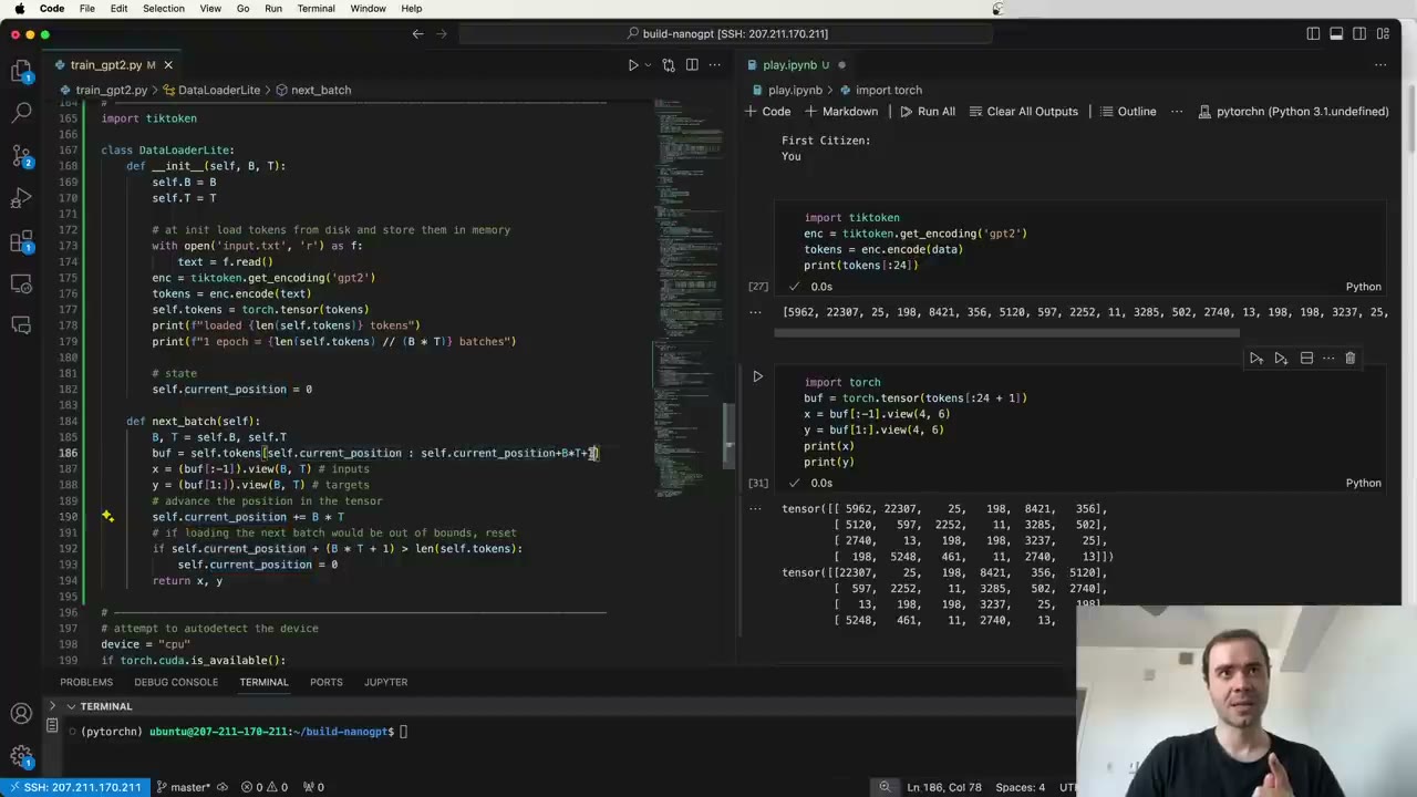
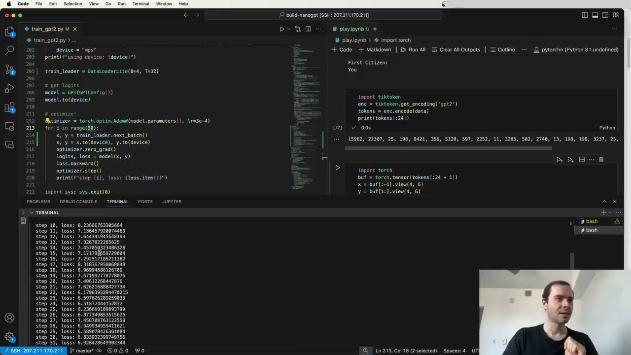
DataLoaderLite then walks the whole file in chunks of B·T tokens, fetching one extra each time and wrapping to the start at the end (1:01:38). He predicts the result before running it (1:04:44): most early gains come from learning that most of the 50,257 tokens never appear in Shakespeare. The file has 338,000 tokens, an epoch is about 2,600 batches at B=4 and T=32, and 50 steps bring the loss to about 6.6 (1:05:47).
1:06:18 – 1:13:27 Weight tying
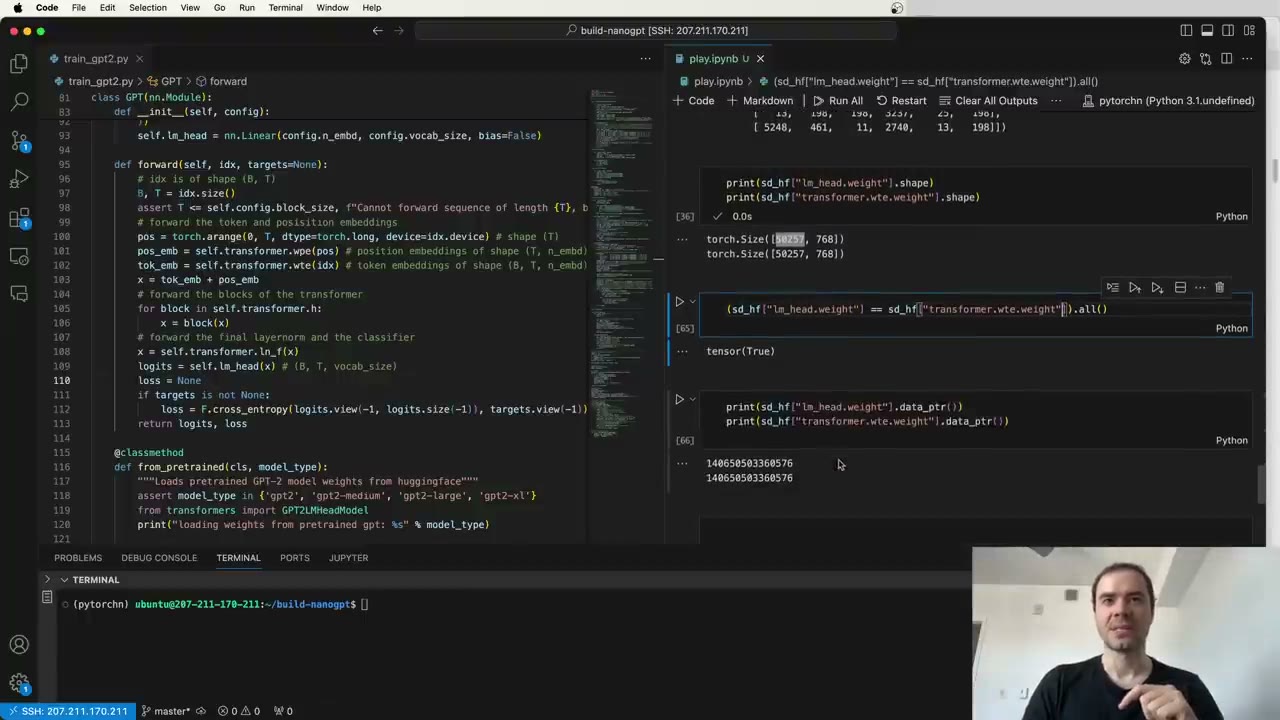
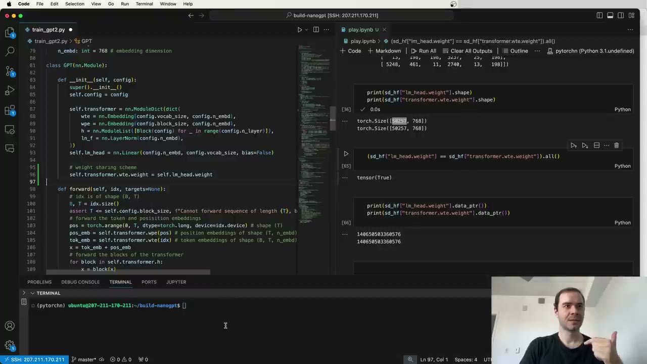
A detail missed in the weight loading: in the Hugging Face state dict, the token embedding and the lm_head weight have the same shape, the same values and even the same data pointer (1:06:50). They are one tensor (1:07:51).
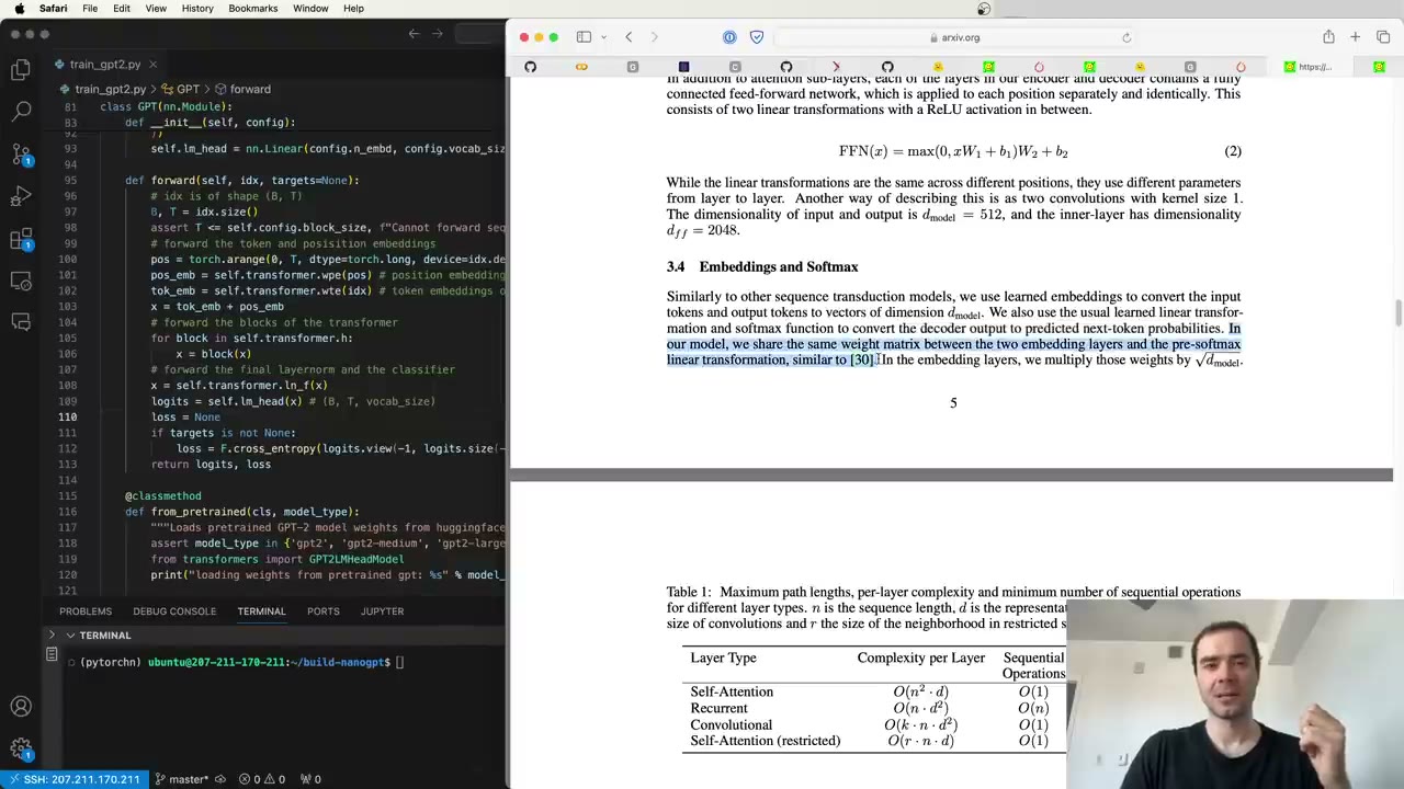
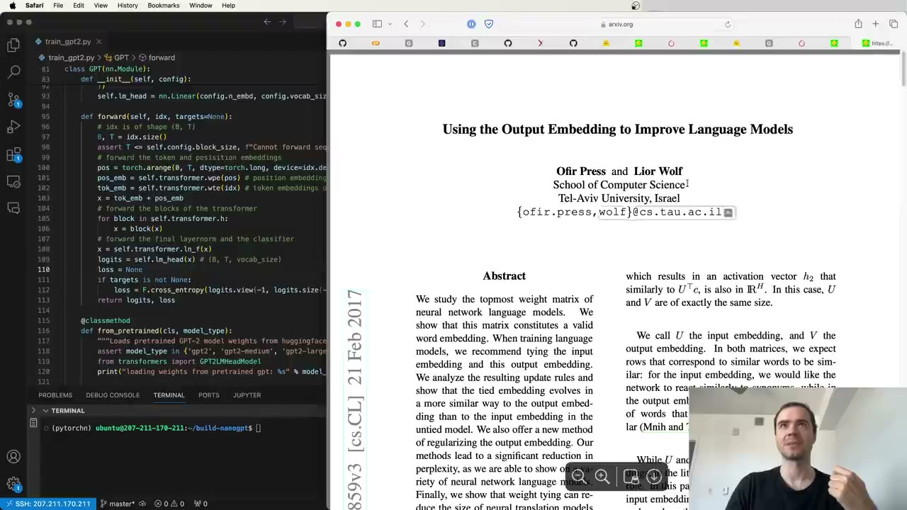
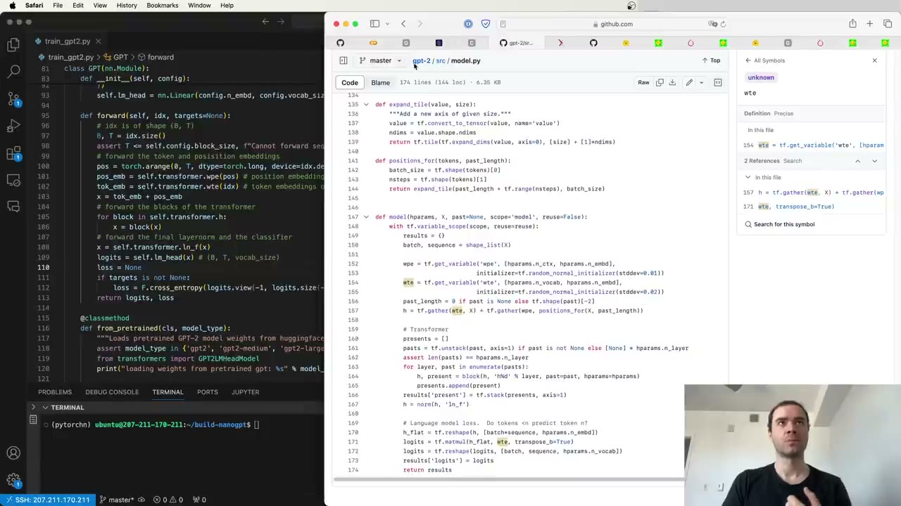
This weight-tying scheme comes from the “Attention Is All You Need” paper and a 2017 paper it cites (1:08:22). The intuition (1:08:53): two tokens that mean nearly the same thing, such as one word in upper and lower case, should sit close together in the input embedding and should also get similar probabilities at the output. Both ends of the network want the same notion of similarity, so let them share it. OpenAI’s TensorFlow code reuses wte to compute the logits (1:10:24), and in the backward pass the gradients from both uses add up on the one tensor (1:10:54).
The fix is a single assignment that points wte.weight at lm_head.weight (1:11:56). The saving is large: 768 × 50,257 is about 40 million parameters, around 30% of the model (1:12:57), which may also help when training time is short.
Our note: the 2017 reference is Press and Wolf, “Using the Output Embedding to Improve Language Models”.
1:13:27 – 1:22:16 Matching GPT-2’s initialization
The papers say little about initialization, so Karpathy reads OpenAI’s model.py (1:13:58): weights drawn from a normal distribution with standard deviation 0.02, biases at zero, token embeddings at 0.02 and position embeddings at 0.01. His _init_weights, run on every submodule through self.apply, does the same, except that he uses 0.02 for both embeddings (1:15:02). Zeroing the biases matters because PyTorch’s default is uniform (1:15:33). LayerNorm’s defaults, scale 1 and offset 0, are already right.
Is a fixed 0.02 reasonable? Xavier-style initialization would use 1/√(fan-in), and for GPT-2’s widths of 768 to 1,600 that lands around 0.02 to 0.03 (1:16:36). So it is roughly in range, though ideally it would shrink as the model grows.
The GPT-2 paper does mention one rule: scale the weights of residual layers by 1/√N, where N is the number of residual layers (1:17:08). Karpathy shows why. Add 100 random unit-variance vectors to a stream and its standard deviation grows to 10; scale each contribution by 1/√100 and it stays at 1 (1:18:09). He marks the projection at the end of each attention and MLP sublayer with a NANOGPT_SCALE_INIT flag (1:19:42) and multiplies their standard deviation by (2 · n_layer)^−0.5 (1:20:44). The 2 is there because each layer adds to the stream twice. The tied embedding gets initialized twice, once as an embedding and once as a linear layer, both at 0.02, which is harmless (1:21:16).
1:22:16 – 1:36:50 Hardware, precision and a speed baseline
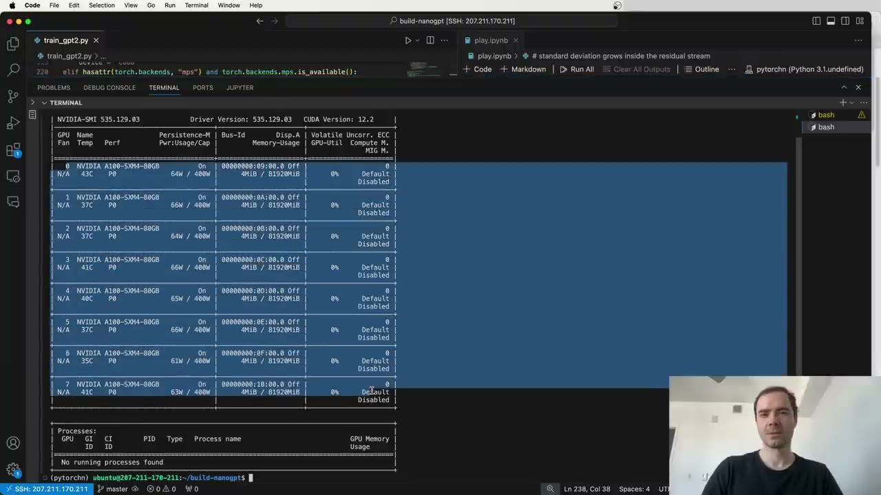
Now the goal is to get full value from the hardware (1:22:16). nvidia-smi shows eight A100 SXM 80GB GPUs, rented from Lambda Labs, which he discloses sponsors his work (1:22:48).
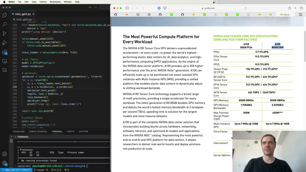
By default every PyTorch tensor is float32 (1:23:50), and deep learning can tolerate much less precision than that. The A100 spec sheet gives 19.5 TFLOPS in FP32, about 8x more with TF32, and 16x (312 TFLOPS) with FP16 or BF16 (1:25:23). Ignore the higher numbers marked with an asterisk, which assume sparsity. INT8 is for inference only, because training needs floating point to represent roughly normal distributions of weights and activations (1:25:55).
Fewer bits also means less memory traffic, and memory bandwidth is the scarce resource (1:26:58). Many training workloads are memory-bound: the tensor cores sit idle waiting for data, and 60% utilization counts as very good (1:27:29).
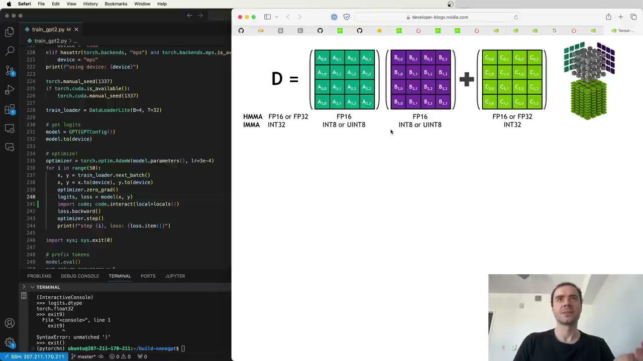
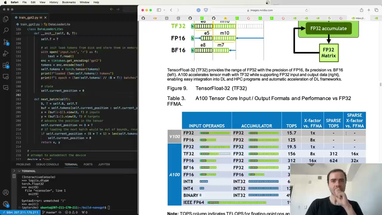
A tensor core is an instruction that multiplies small 4×4 matrices (1:28:00), and every matrix multiply is broken into these. Almost all of a Transformer’s compute is matrix multiplication, and at this size the largest single one is the classifier from 768 to 50,257 (1:29:32). TF32 keeps float32’s sign and 8 exponent bits but cuts the mantissa, so 19 bits are used inside the instruction while inputs and outputs stay FP32 (1:31:06). Your code sees no difference.
The baseline uses B=16 and the real sequence length T=1024 (1:32:39). Timing GPU work needs torch.cuda.synchronize(), because the CPU only queues kernels and would otherwise stop the clock before the GPU has finished (1:33:43). The result is about 1,000 ms per step using 35 GB of memory, with a slower first iteration while PyTorch sets up (1:34:47). If you run out of memory, shrink the batch, but keep to numbers with many factors of two (1:35:48). From here he reports tokens per second as the real throughput measure (1:36:18).
Our note: the terminal shows about 1,003 ms and about 16,300 tokens per second per step (16 × 1,024 tokens). The captions’ “163,000” is a mis-hearing.
1:36:50 – 1:48:25 TF32 and bfloat16
Enabling TF32 is one line, torch.set_float32_matmul_precision('high') (1:36:50), on Ampere GPUs or newer. The promised 8x turns into about 3x, from 1,000 ms to about 333 ms and roughly 50,000 tokens per second (1:38:24), because every number moving through memory is still 32 bits (1:38:57).
The next step halves that traffic with bfloat16 (1:39:59). The key difference from FP16 (1:40:30): BF16 keeps float32’s 8 exponent bits, so it covers the same range of values with less precision inside it. FP16 shrinks the range as well, which is why FP16 training, the norm on the older Volta GPUs, needed gradient scalers (1:41:32). BF16 arrived with Ampere and needs none of that (1:42:03).
Following the PyTorch mixed-precision guide, which he says is the clearest of several, he wraps only the forward pass and the loss in torch.autocast(device_type='cuda', dtype=torch.bfloat16) and leaves the backward pass and optimizer step alone (1:43:39). The logits now come out as bfloat16 while the parameters stay float32 (1:44:40), hence mixed precision. Matrix multiplies are cast down, while softmax, LayerNorm and loss calculations may stay in float32 because they are more sensitive (1:45:44). The gain is modest: 333 ms to 300 ms, about 55,000 tokens per second (1:46:51). The precision loss is usually worth it, since the time saved can go into training longer (1:47:53).
1:48:25 – 2:00:19 torch.compile and the GPU memory hierarchy
torch.compile is, in his description, something like GCC for neural networks (1:48:25). One line, model = torch.compile(model), costs some compile time up front and takes a step from 300 ms to 129 ms, about 2.3x (1:49:26). He suggests using it by default unless you are debugging.
Where the speed comes from (1:50:26). In normal “eager” mode, the Python interpreter runs one operation at a time with no idea what comes next. The compiler sees the whole forward pass at once, removes Python from it (1:50:58), and can reorganize the work.
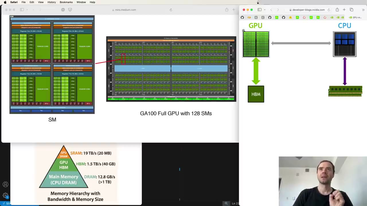
His example is the tanh GELU written out by hand (1:51:32). In eager mode, cubing the input sends the whole tensor from GPU memory (HBM) to the chip and back; multiplying by a constant does the round trip again, adding the input again, and so on (1:53:05). The compiler sees these are all element-wise operations and fuses them into one kernel: load each chunk once, do every step on chip, write once (1:54:37). That is kernel fusion, and it brings throughput to about 125,000 tokens per second (1:55:39).
He fills in the hardware picture (1:56:42). HBM is a separate chip holding tens of gigabytes. The GPU die has many streaming multiprocessors (SMs), each with tensor cores and other arithmetic units, plus small on-chip memories: L2 cache, L1 cache and registers, built as SRAM (1:57:13). On-chip memory is very fast but totals only a few tens of megabytes (1:58:14). Every unfused kernel streams data from HBM to the chip and back, and fusion keeps a chunk on chip while it does all its work (1:59:48).
Our note: Karpathy says the chip has about 120 SMs. NVIDIA’s full GA100 diagram shows 128, of which the shipping A100 enables 108.
2:00:19 – 2:06:39 FlashAttention
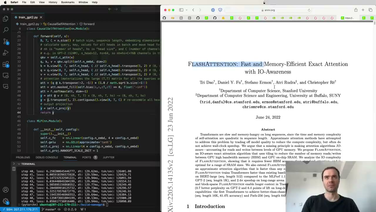
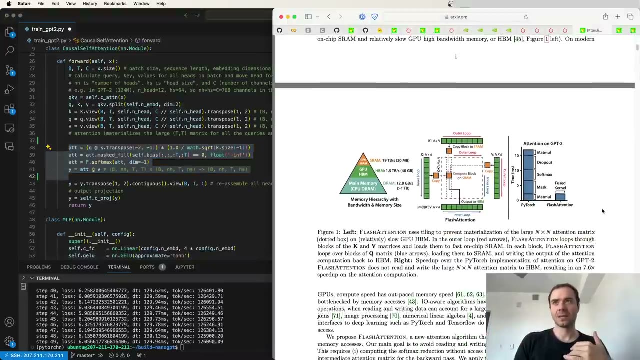
Some fusions are beyond the compiler. FlashAttention, from a 2022 Stanford paper, replaces the four lines of attention (scores, mask, softmax, weighted sum) with a single fused kernel (2:00:19). torch.compile cannot find it because it requires rewriting the algorithm (2:01:22). It actually does more FLOPs than standard attention, yet the paper reports it running up to 7.6x faster, because it never writes the T×T attention matrix out to HBM (2:01:53). For one head of one sequence that matrix is already a million numbers (2:02:25).
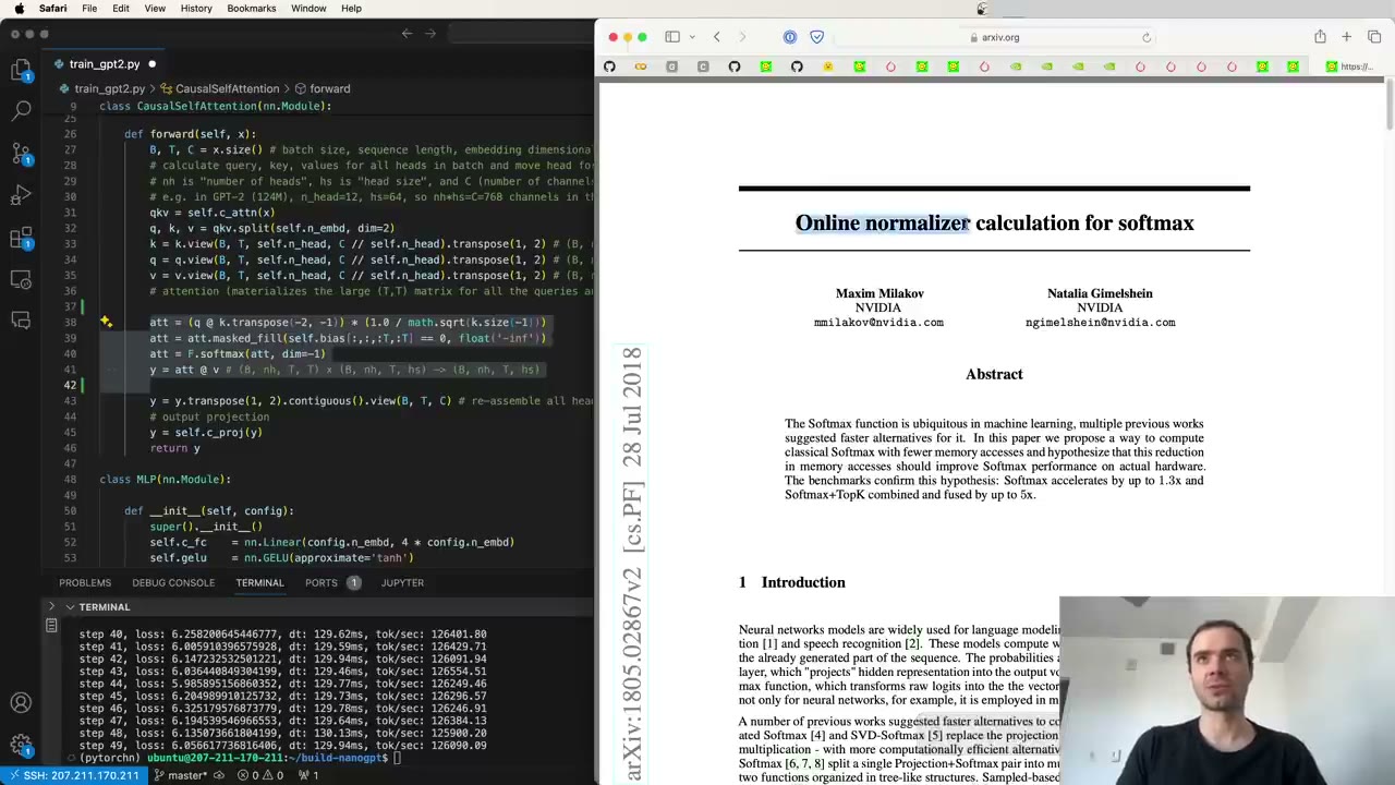
The enabling trick is the online softmax (2:02:57). By keeping a running maximum and a running sum, you can compute a softmax in a single streaming pass without seeing all its inputs first. Karpathy finds it striking that this came from an NVIDIA paper in 2018, four years before FlashAttention, which predicted the memory savings but did not take the next step (2:03:30). His lesson: the pattern of memory access matters more than the FLOP count (2:04:33).
In PyTorch it is one call, F.scaled_dot_product_attention(q, k, v, is_causal=True) (2:05:04). The loss after 50 steps is the same up to floating-point noise, and the step drops from about 130 ms to about 96 ms, roughly a 27% gain (2:06:07).
2:06:39 – 2:14:58 Nice numbers: padding the vocabulary
Karpathy calls the next one “the dumbest and the most brilliant optimization” (2:06:39). CUDA kernels work in tiles sized in powers of two, so sizes like 64, 128 and 256 are “nice” and odd or prime sizes are “ugly” (2:07:10). He scans the config: 768 and 1,024 are fine, 50,257 is very ugly (2:08:12), and GPT-2 XL’s 25 heads caused his team real trouble when optimizing kernels (2:08:43).
The fix is to round the vocabulary up to 50,304, which divides by 128 (2:09:13). This adds work, yet a step drops from 96.5 ms to 93 ms, about 4% (2:10:49). Is it safe (2:11:19)? The extra embedding rows are never indexed, because the tokenizer never produces those ids. Through weight tying they do become extra output logits, but the network learns to push them toward zero probability, just as it does for the tens of thousands of real tokens that never appear in Shakespeare (2:12:21).
Why faster: kernels process the evenly tiled part of a tensor first, then run a separate, inefficient pass for the leftover edge (2:12:53). Padding removes the leftover. On PyTorch 2.3.1 or earlier, Karpathy says, the same change gives about 30% (2:14:27). Running total: about 11x, from 1,000 ms to 93 ms per step (2:14:58).
2:14:58 – 2:25:57 GPT-3’s optimizer recipe
Now the algorithm itself. OpenAI released GPT-2’s weights and inference code but no training code, and the paper is vague (2:15:30). GPT-3 is the opposite: detailed paper, no weights. The architectures are close enough to borrow from (GPT-3 mainly doubles the context to 2,048), so the GPT-3 appendix becomes the guide (2:16:02).
- AdamW settings (2:16:34). Betas of 0.9 and 0.95 instead of PyTorch’s default 0.999 for the second, and epsilon 1e-8.
- Gradient clipping at 1.0 (2:17:04). After
backward(), the global norm of all gradients (square everything, sum, square root) is capped at 1.0, which protects the model from a sudden shock caused by an unlucky batch (2:18:07). He calls it a bit of a hack.clip_grad_norm_returns the norm, and he prints it every step: a climbing norm or spikes mean instability (2:19:08). In his run it starts near 30 and settles below 1 (2:20:11).
- Cosine decay with linear warmup (2:20:44). GPT-3 warms up over the first 375 million tokens and decays to 10% of the peak over 260 billion tokens (2:21:14). He writes his own
get_lrrather than using PyTorch’s schedulers, because it is five lines he fully understands (2:22:49). Setting the rate means looping over the optimizer’sparam_groups(2:22:18). The peak becomes 6e-4, from GPT-3’s table for its 125M “Small” model (2:23:19), andit + 1in the warmup avoids a learning rate of exactly zero on step 0 (2:24:22).
One knowing deviation: GPT-3 finished decaying at 260B tokens and trained on at 10% until 300B, while here the decay runs to the final step (2:25:26). Which schedule is best is, he says, still an open research question.
2:25:57 – 2:34:49 Batch ramp, weight decay and fused AdamW
GPT-3 also ramps the batch size up gradually (2:25:57). Karpathy skips it. It complicates the token arithmetic, and he sees it as a speed trick rather than an algorithmic gain (2:26:29). Early in training every example says much the same thing, mostly which tokens never occur, so the gradients are highly correlated and a small batch gives the same signal as a huge one (2:27:30). Sampling without replacement within an epoch is already what the sequential loader does (2:28:32).
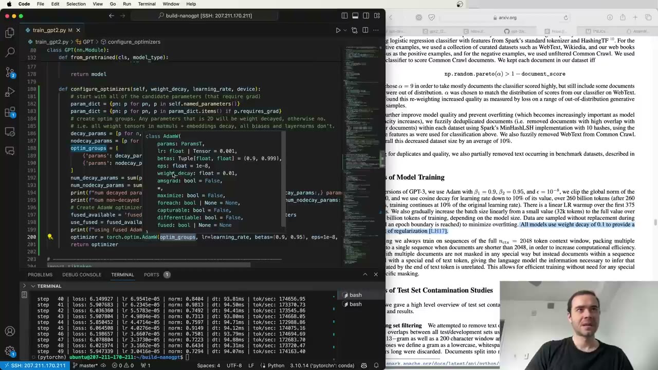
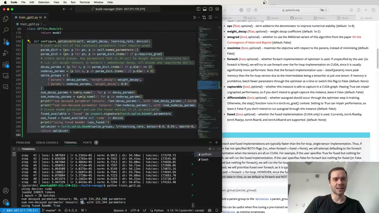
Weight decay of 0.1 goes in a new configure_optimizers method (2:29:03). That is ten times AdamW’s default of 0.01 (2:29:34). Only parameters with two or more dimensions are decayed: the matrices in linear layers and the embeddings. Biases and LayerNorm parameters are not (2:30:05). The idea is a gentle pull toward zero that keeps any single weight from growing large and pushes the network to spread work over more channels (2:30:36). The split works out to 50 decayed tensors and 98 non-decayed ones, the latter only about 121,000 parameters (2:32:42).
The same method turns on fused=True for AdamW when the installed PyTorch supports it, checked with inspect (2:31:38). Fused AdamW updates all parameters in one kernel rather than looping over tensors, a kernel fusion for the optimizer (2:32:10). Step time drops from 93 to 90 ms (2:33:13). He adds that the interactions between weight decay, learning rate, batch size and Adam’s settings are a deep subject he is deliberately not covering (2:33:46).
2:34:49 – 2:46:43 Gradient accumulation
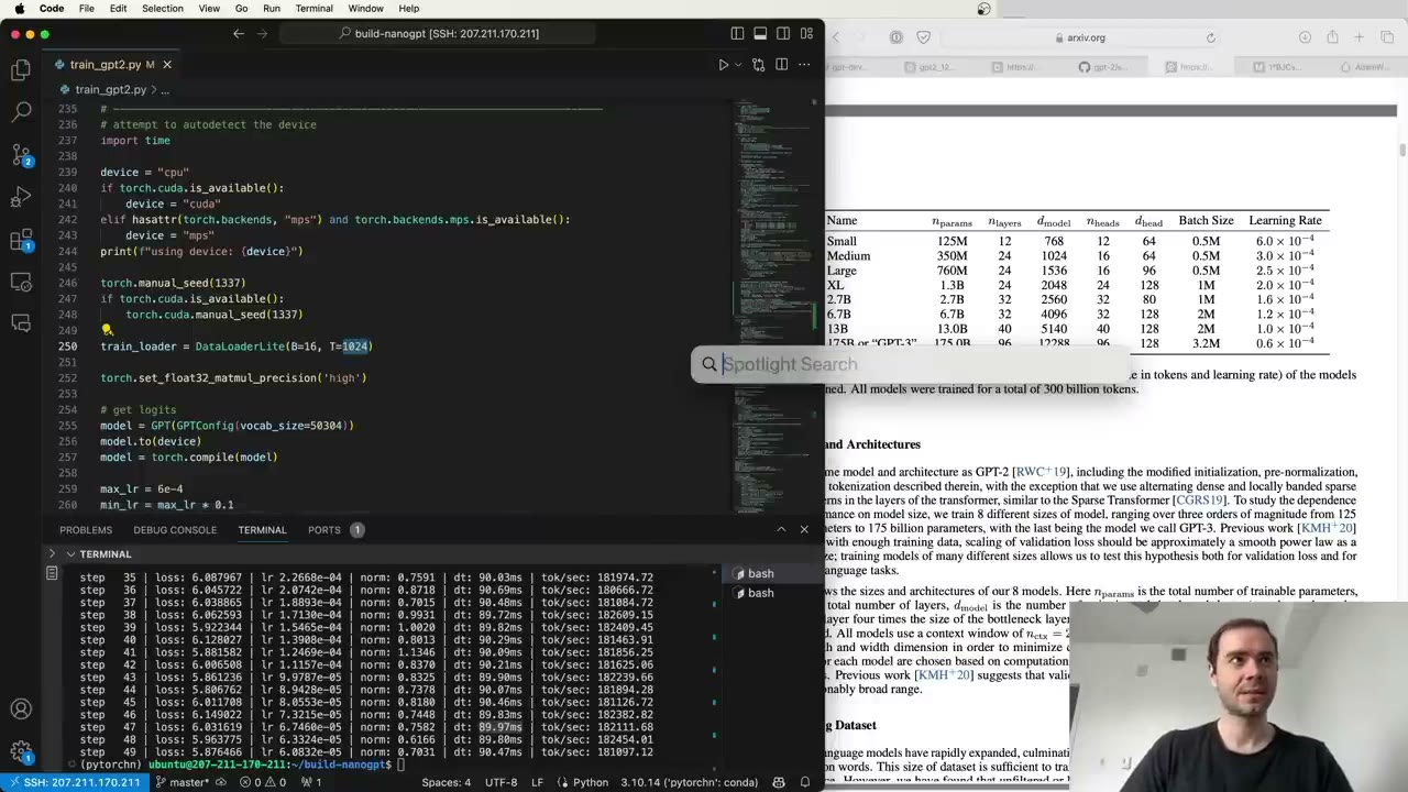
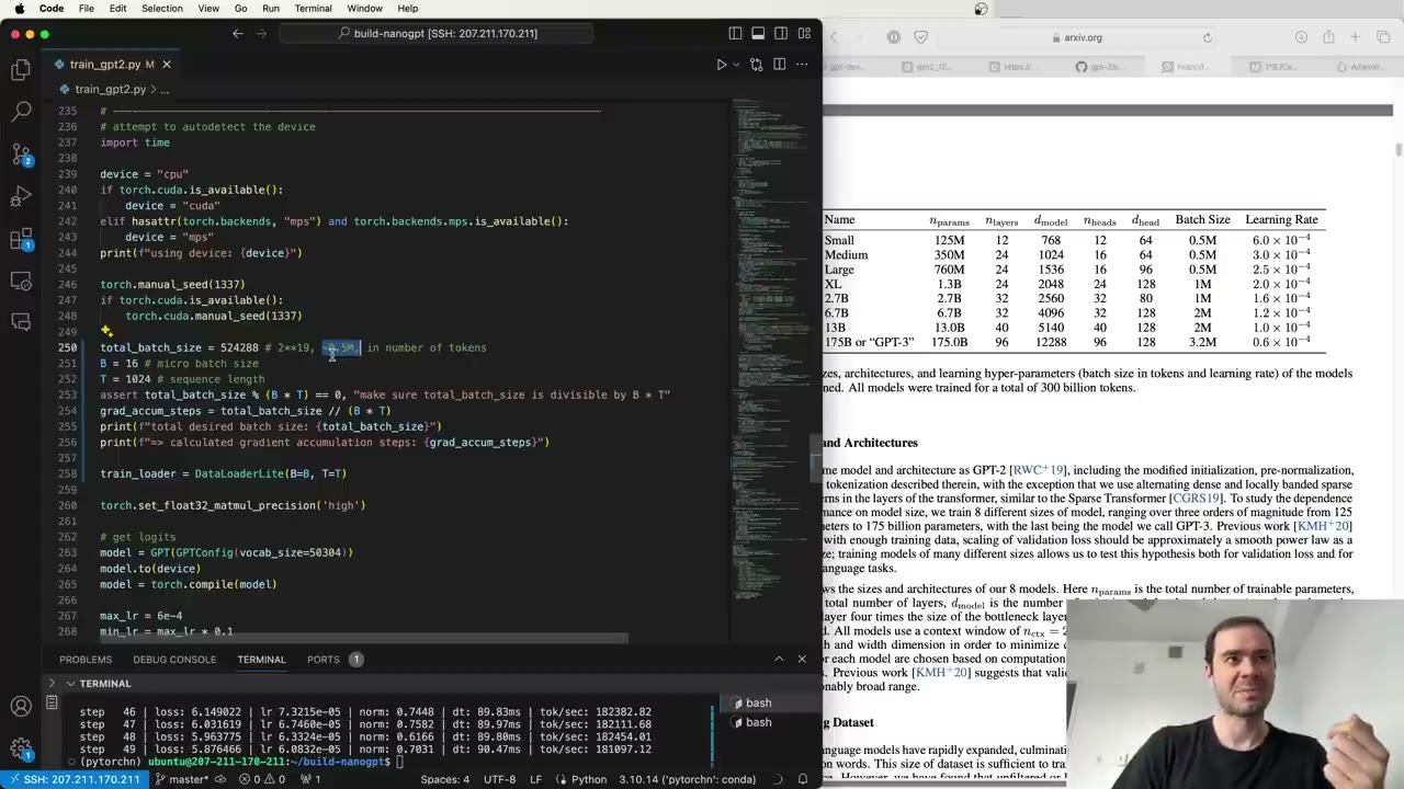
GPT-3 Small trained with a batch of about 0.5 million tokens (2:34:49). At 1,024 tokens per row that is around 488 rows, which no single GPU can hold (2:35:51). Batch size interacts with the other hyperparameters, so to use GPT-3’s settings faithfully you need that batch, and gradient accumulation simulates it by running several forward and backward passes before each update (2:36:22).
The total is set to 2^19 = 524,288 tokens, a nice number close to half a million (2:36:54). With micro-batches of 16 × 1,024 tokens that is 32 micro-steps, about 3 seconds per optimizer step (2:38:28).
The obvious inner loop has a subtle bug, and he invites you to spot it (2:39:29). A toy notebook shows it (2:39:59). A tiny regression net with mean-squared error over four examples gives one gradient; four accumulation steps of one example each give a different one (2:42:03). The mean loss carries a factor of 1/4. Accumulating gradients is equivalent to summing losses, so that factor disappears (2:42:33). Dividing each loss by 4 makes the gradients match (2:43:04). Cross-entropy is a mean too, so in the training loop the fix is loss = loss / grad_accum_steps (2:44:08).
For logging he adds a loss_accum that sums the detached, already-scaled losses (2:45:09), and counts tokens per step as B × T × grad_accum_steps. A useful consequence: B is now purely a performance setting. Any value that fits your GPU should give the same optimization up to floating-point error (2:46:12).
2:46:43 – 2:59:25 Going multi-GPU with DDP
Time to use all eight GPUs with PyTorch’s DistributedDataParallel; he advises against the legacy DataParallel (2:46:43). The model is simple: eight processes, one per GPU, each running the same training code on a different slice of data, and the gradients are averaged before each update (2:47:45).
The script is launched with torchrun, which starts the copies and sets RANK, LOCAL_RANK and WORLD_SIZE environment variables in each (2:48:16). The rank is the only thing that differs between processes (2:49:19). The local rank picks the GPU, as in cuda:3 (2:50:23), and rank 0 is the “master process” that handles printing, logging and checkpoints (2:50:55). Without torchrun the code falls back to one GPU. His advice for reading such code: picture eight Python interpreters going down the same lines at once (2:51:25).
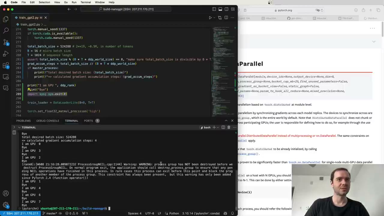
Accumulation steps now divide by the number of GPUs too: 524,288 / (16 × 1,024 × 8) = 4 (2:52:58). Prints are guarded by master_process so they don’t appear eight times (2:53:30). A quick test with torchrun --standalone --nproc_per_node=8 train_gpt2.py shows the processes finishing in arbitrary order, and a complaint because destroy_process_group() was never called (2:56:14).
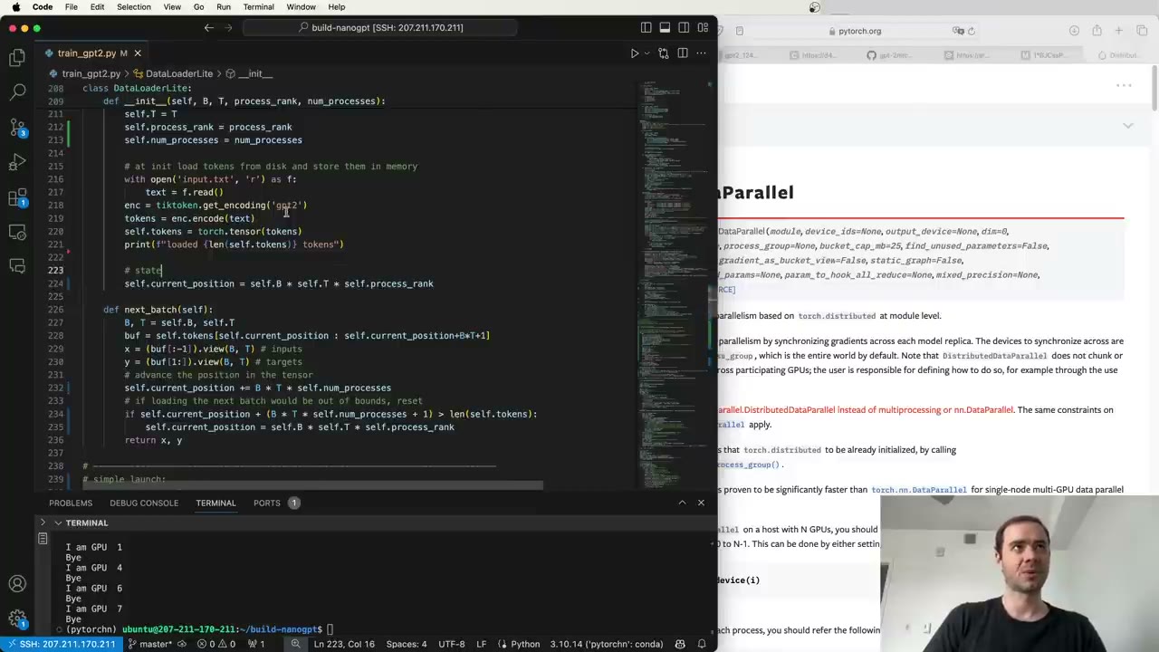
The data loader needs to know its place (2:56:45). Each process starts at offset B·T·rank and advances by B·T·world_size, so the eight processes read interleaved, non-overlapping chunks (2:57:49). With one process this reduces to the old loader. Every process builds an identical model because they share the random seed (2:58:54).
2:59:25 – 3:10:20 Synchronizing gradients and losses
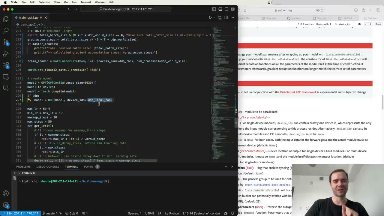
The model is wrapped as DDP(model, device_ids=[ddp_local_rank]) (2:59:55); he finds the documentation for device_ids unclear but is fairly sure it wants the local rank (3:00:26). The forward pass is unchanged. At the end of the backward pass, DDP runs an all-reduce that averages every gradient across ranks and leaves the result on all of them (3:00:56), and it overlaps that communication with the backward computation (3:01:27).
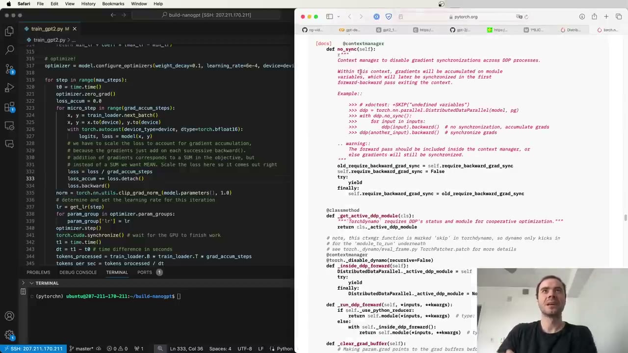
With accumulation you only want that sync on the last micro-step (3:01:57). The official route is the no_sync() context manager, which he dislikes because it duplicates code (3:02:58). Reading its source, he finds it only flips a flag, so he sets model.require_backward_grad_sync directly to true on the last micro-step and false otherwise (3:04:01). He admits this relies on an internal that could change.
DDP averages gradients but not the logged loss, so loss_accum gets its own dist.all_reduce(..., op=dist.ReduceOp.AVG) (3:05:35). The token count is multiplied by the world size, and the process group is destroyed at exit (3:07:10). The result: about 1.5 million tokens per second (3:07:43). One more fix: the optimizer is configured through raw_model = model.module, since the DDP wrapper does not expose the method (3:08:15).
Single-GPU and eight-GPU losses don’t match exactly (3:08:46). The reason is mundane: the loaders wrap around the file at different points. With a small total batch (32,768 tokens) the boundary effects shrink and the numbers line up (3:09:48).
3:10:20 – 3:17:42 Choosing a dataset: FineWeb-Edu
Tiny Shakespeare is outgrown. GPT-2 trained on WebText, pages behind Reddit outbound links with at least 3 karma, about 45 million links and 40 GB of text, never released; OpenWebText is an attempt to recreate it (3:10:20). GPT-3 added Common Crawl, which Karpathy warns is far noisier than people assume, full of spam, tables and stock tickers, so it is heavily filtered and mixed with sources such as WebText, books and Wikipedia (3:10:54). Public stand-ins include RedPajama and its cleaned, deduplicated subset SlimPajama (3:11:56).
His pick is FineWeb, a 15-trillion-token filtered Common Crawl, and specifically FineWeb-Edu, Hugging Face’s educational subset (1.3T tokens at the stricter threshold, 5.4T at the looser one) (3:12:27). He uses the 10-billion-token sample, which in his earlier experiments was enough to get close to GPT-2 (3:13:28). The filtering was done automatically by Llama 3 70B judging which pages are educational (3:15:04).
fineweb.py downloads the data, tokenizes every document with <|endoftext|> (id 50256) placed at the start, stores tokens as uint16 since every id fits under 65,536 (3:16:06), and writes NumPy shards of exactly 100 million tokens (3:16:39). Shard 0 is validation. Sharding keeps files manageable, and the whole job takes about 30 minutes (3:17:12).
3:17:42 – 3:22:33 Launching the real run
The folder now holds 100 shards, 10 billion tokens (3:17:42). The loader learns to load shards, convert them to long tensors, move to the next shard when one runs out, and take a split argument for train or val (3:18:14).
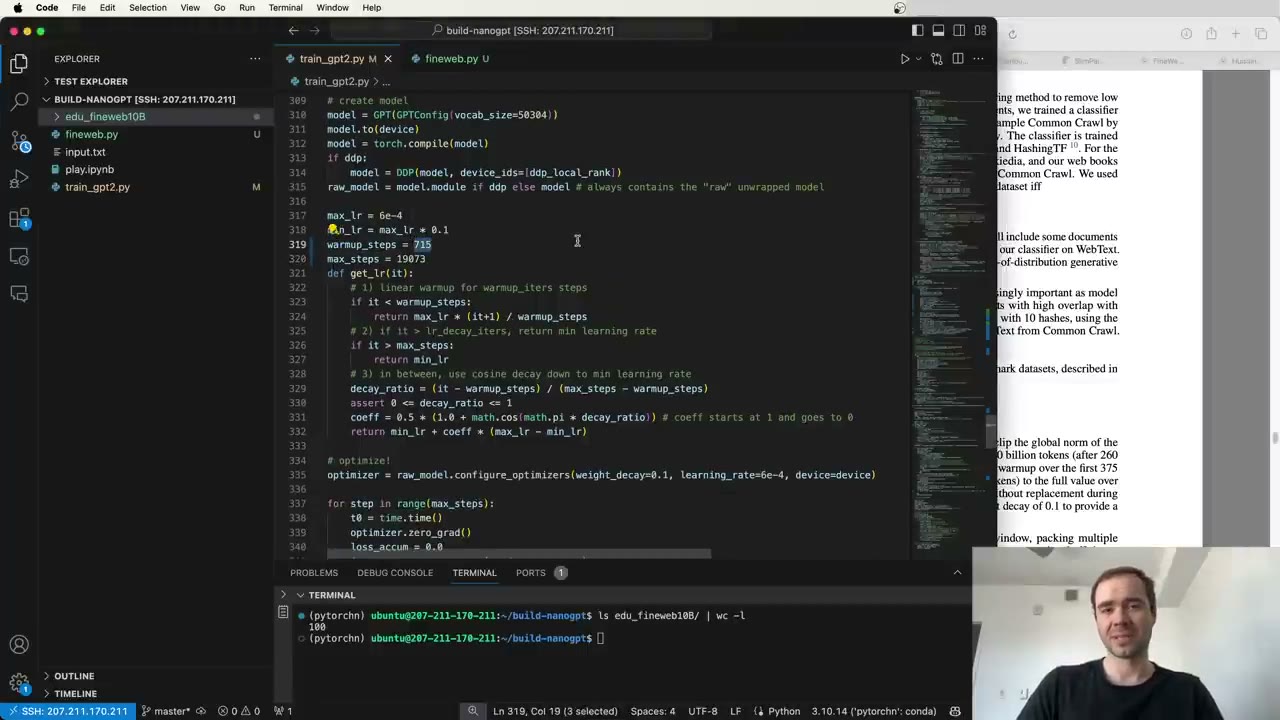
The schedule follows from the batch size (3:19:17). Ten billion tokens at 2^19 per step is 19,073 steps, one epoch. GPT-3’s 375 million warmup tokens become 715 steps (3:19:47), which he thinks is very mild; around 100 would probably do, but he keeps GPT-3’s value. On his 80 GB cards a micro-batch of 64 fits (3:20:18), and 64 × 1,024 × 8 GPUs is the full 524,288 tokens, so no accumulation is needed (3:20:50). At about 1.5 million tokens per second and 330 ms per step, one epoch takes about 1.7 hours (3:22:03).
3:22:33 – 3:28:16 Validation loss and sampling during training
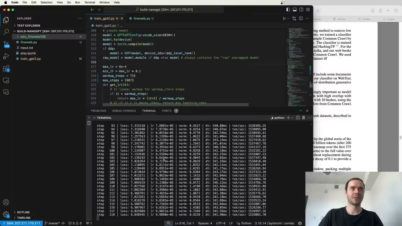
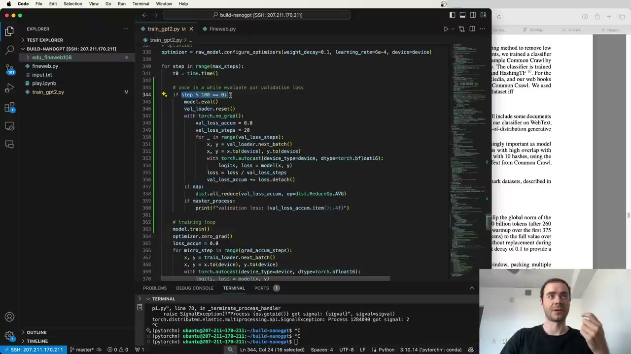
Before the real run, evaluation and logging (3:22:33). A validation loader reads shard 0, and a new reset() method rewinds it. Every 100 steps the model switches to eval mode and averages the loss over 20 validation batches with no backward pass (3:23:37). With effectively unlimited data, train and validation loss should track each other (3:24:07), but the validation split becomes essential once you train for several epochs and could memorize (3:25:11). It also allows a reference point: run the released GPT-2 124M on the same validation data (3:24:39).
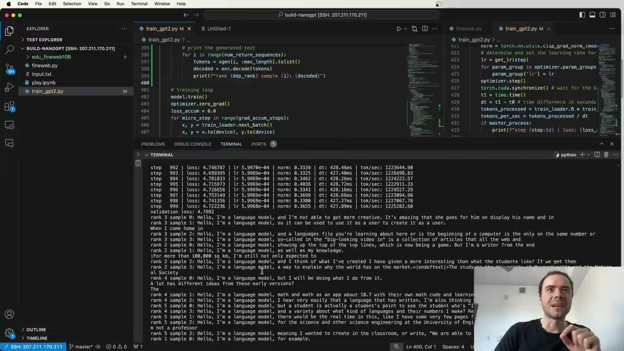
The old sampling code moves into the loop and runs periodically. It uses its own torch.Generator, seeded differently per rank, so sampling never disturbs the random state used for training (3:26:44). At step 1,000 the samples are still mostly garbled; the model is, in his words, “still a young baby” (3:26:14). One wart: with torch.compile on, sampling crashed with an error he couldn’t resolve, so compile is off for these runs (3:27:14). He mentions he committed at every stage, so the build-nanogpt history follows the video step by step (3:27:45).
3:28:16 – 3:41:50 Evaluating with HellaSwag
Validation loss on FineWeb-Edu is not a fair comparison with a model trained on different data, so he adds HellaSwag, a 2019 benchmark (3:28:16). Each item is a short context and four possible endings, one natural and three wrong (3:28:47). The contexts come from ActivityNet and WikiHow, covering a broad range of everyday knowledge (3:29:50). The wrong endings were generated adversarially by language models to be easy for people and hard for models: humans scored about 95%, the best models of the day about 48% (3:30:22). Today’s models score about 96%, so it is essentially solved (3:30:54). It stays popular because it is smooth and gives early signal: even tiny models climb slowly up from the 25% chance level (3:31:59).
Small models cannot handle a lettered multiple-choice format, so the task is posed as token completion (3:32:29). Build four rows, each the shared context followed by one ending, padded to the same length, with a mask marking the ending tokens (3:33:30). The prediction is the ending whose tokens get the lowest average cross-entropy loss, which he believes is how GPT-3 did it (3:34:01). This is harder than formats where the model sees all four options at once (3:35:05).
hellaswag.py downloads the 10,000 validation examples and renders them this way (3:35:36). Baselines: GPT-2 124M scores 29.55% and GPT-2 XL about 49% (3:37:11). The EleutherAI evaluation harness reports slightly different numbers, possibly because it uses the multiple-choice style (3:37:42).
In the training script (3:38:45): compile is off by default because it breaks this evaluation as well. A log.txt records train loss, validation loss and HellaSwag accuracy (3:39:15). Validation, HellaSwag and sampling run every 250 steps and on the last step (3:39:46). The GPUs split HellaSwag examples by index modulo world size, and their counts are combined with an all-reduce sum (3:40:48).
3:41:50 – 3:53:37 Results: one epoch and an overnight run
Halfway through, at step 10,000 of about 20,000, the samples are getting less random and more on-topic (3:41:50).
“Good morning.” The finished one-epoch run is plotted in a notebook (3:43:03). It ran 19,073 steps, about 10 billion tokens (3:43:41). Validation loss ends below the released GPT-2 124M’s loss on the same validation data, though Karpathy repeats that the data distributions differ (3:44:13). On HellaSwag the model climbs from 25% past GPT-2 124M’s line, with the GPT-3 124M model (trained on 300 billion tokens) still above it (3:44:44).
Matching GPT-2 with 10 billion tokens against its 100 billion needs explaining, and he offers several possibilities (3:45:14):
- FineWeb-Edu is English-only with little math or code, while GPT-2’s data may have spent capacity on those.
- HellaSwag is five years old and could have leaked into the training data, though the FineWeb-Edu team used it as an eval and probably deduplicated against it (3:45:45).
- Today’s datasets get far more careful filtering and deduplication, so each token may simply be worth more (3:47:50).
The training loss shows an odd periodic pattern (3:46:48). His suspicion is that the 10B sample is not well shuffled, and since the loader reads it strictly in order, it inherits that ordering.
For the overnight run he multiplied training by four: four epochs, about 40 billion tokens, around eight hours (3:48:20). HellaSwag rose a lot and nearly reached GPT-3 124M (3:49:25), ending at 33.24% after about 76,290 steps (3:52:33). That is roughly a 10x saving in tokens against GPT-3’s 300 billion (3:50:58). The periodicity shows up again at the epoch boundaries, and he says a better loader would shuffle documents within each shard and the order of the shards every epoch, because which document follows which in a row is a spurious correlation (3:49:56).
Two more pointers. Others have found that the maximum learning rate can be roughly tripled, so GPT-3’s settings may be conservative (3:51:29). And to match GPT-3 exactly, use T = 2,048 and B = 32 to keep half a million tokens per step (3:52:01). The overnight model’s samples are noticeably more coherent (3:53:06).
Our note: the GPT-3 paper reports 33.7% zero-shot HellaSwag for its 125M model (shown on screen at 3:31:47), which is the upper dashed line he compares against.
3:53:37 – 3:59:21 Checkpoints, fine-tuning and llm.c
Every 5,000 steps the master process now saves a checkpoint, the model’s state dict (3:53:37). To resume training exactly you would also need the optimizer state (AdamW’s m and v buffers) and the random number generator states (3:54:09). Checkpoints also let you run fuller evaluations later, for example with the EleutherAI harness on math, code or other languages (3:54:40).
Everything so far is pretraining. The model, as he puts it, dreams documents; you cannot chat with it (3:55:13). Supervised fine-tuning is not much deeper than swapping in a conversational dataset with user and assistant turns and continuing to train (3:55:44).
He ends with llm.c, his pure CUDA implementation of GPT-2 and GPT-3 training (3:56:15), which uses a nanoGPT-style PyTorch script as its reference (3:56:47). Run side by side on one GPU each, llm.c compiles and starts much sooner than torch.compile (3:57:49), runs at about 223,000 tokens per second against PyTorch’s 185,000, and prints losses and gradient norms that line up step for step (on screen they agree to about four decimal places) (3:58:49). He notes the comparison is not quite fair: PyTorch is a general framework, and he may not have tuned it fully.
3:59:21 – end Wrap-up and open issues
The summary (3:59:21): from the GPT-2 and GPT-3 papers and a blank file, a two-hour run matches GPT-2 124M and an overnight run nearly matches GPT-3 124M, and the same code could train bigger models given the patience or compute (3:59:55). Open items he lists (4:00:26): the periodic loss, torch.compile breaking sampling and HellaSwag, and permuting the data at epoch boundaries. He points to the build-nanogpt repo’s discussions and issues, and the Zero to Hero Discord (4:00:57).
Our note: the build-nanogpt README and commit history are the place to check how these issues were handled after the video.
Code you’ll write
These are short excerpts in the style of train_gpt2.py, which follows the code built in the video. The full, MIT-licensed code, with one commit per step of the lecture, is in karpathy/build-nanogpt, and the longer-lived version is karpathy/nanoGPT.
The Block and MLP (17:43). Pre-norm residual block: LayerNorm feeds each sublayer, and the residual stream itself is only ever added to.
class MLP(nn.Module):
    def __init__(self, config):
        super().__init__()
        self.c_fc = nn.Linear(config.n_embd, 4 * config.n_embd)
        self.gelu = nn.GELU(approximate='tanh')
        self.c_proj = nn.Linear(4 * config.n_embd, config.n_embd)
        self.c_proj.NANOGPT_SCALE_INIT = 1

    def forward(self, x):
        x = self.c_fc(x)
        x = self.gelu(x)
        x = self.c_proj(x)
        return x

class Block(nn.Module):
    def __init__(self, config):
        super().__init__()
        self.ln_1 = nn.LayerNorm(config.n_embd)
        self.attn = CausalSelfAttention(config)
        self.ln_2 = nn.LayerNorm(config.n_embd)
        self.mlp = MLP(config)

    def forward(self, x):
        x = x + self.attn(self.ln_1(x))  # communicate
        x = x + self.mlp(self.ln_2(x))   # compute per token
        return x
Causal self-attention with FlashAttention (23:57, swapped to the fused call at 2:05:04). One linear layer makes q, k and v for every head; heads become a batch dimension.
def forward(self, x):
    B, T, C = x.size()
    qkv = self.c_attn(x)                       # (B, T, 3 * n_embd)
    q, k, v = qkv.split(self.n_embd, dim=2)
    k = k.view(B, T, self.n_head, C // self.n_head).transpose(1, 2) # (B, nh, T, hs)
    q = q.view(B, T, self.n_head, C // self.n_head).transpose(1, 2) # (B, nh, T, hs)
    v = v.view(B, T, self.n_head, C // self.n_head).transpose(1, 2) # (B, nh, T, hs)
    y = F.scaled_dot_product_attention(q, k, v, is_causal=True) # flash attention
    y = y.transpose(1, 2).contiguous().view(B, T, C) # re-assemble all head outputs
    y = self.c_proj(y)
    return y
Model skeleton, weight tying and GPT-2 initialization (15:08, 1:11:56, 1:19:42). Names match Hugging Face’s state dict; the residual projections get the 1/√(2·n_layer) scaling.
self.transformer = nn.ModuleDict(dict(
    wte = nn.Embedding(config.vocab_size, config.n_embd),
    wpe = nn.Embedding(config.block_size, config.n_embd),
    h = nn.ModuleList([Block(config) for _ in range(config.n_layer)]),
    ln_f = nn.LayerNorm(config.n_embd),
))
self.lm_head = nn.Linear(config.n_embd, config.vocab_size, bias=False)
self.transformer.wte.weight = self.lm_head.weight   # weight tying
self.apply(self._init_weights)

def _init_weights(self, module):
    if isinstance(module, nn.Linear):
        std = 0.02
        if hasattr(module, 'NANOGPT_SCALE_INIT'):
            std *= (2 * self.config.n_layer) ** -0.5
        torch.nn.init.normal_(module.weight, mean=0.0, std=std)
        if module.bias is not None:
            torch.nn.init.zeros_(module.bias)
    elif isinstance(module, nn.Embedding):
        torch.nn.init.normal_(module.weight, mean=0.0, std=0.02)
Forward pass with loss (30:44, loss added at 52:38). Position and token embeddings are added, the blocks run, and cross-entropy is computed on flattened logits.
def forward(self, idx, targets=None):
    B, T = idx.size()
    assert T <= self.config.block_size
    pos = torch.arange(0, T, dtype=torch.long, device=idx.device) # shape (T)
    pos_emb = self.transformer.wpe(pos)        # (T, n_embd)
    tok_emb = self.transformer.wte(idx)        # (B, T, n_embd)
    x = tok_emb + pos_emb
    for block in self.transformer.h:
        x = block(x)
    x = self.transformer.ln_f(x)
    logits = self.lm_head(x)                   # (B, T, vocab_size)
    loss = None
    if targets is not None:
        loss = F.cross_entropy(logits.view(-1, logits.size(-1)), targets.view(-1))
    return logits, loss
Cosine learning-rate schedule with warmup (2:21:46). Linear warmup to 6e-4, cosine decay to 10% of that; the step counts are those of the final run.
max_lr = 6e-4
min_lr = max_lr * 0.1
warmup_steps = 715
max_steps = 19073   # 10B tokens / 2**19 tokens per step

def get_lr(it):
    if it < warmup_steps:
        return max_lr * (it + 1) / warmup_steps
    if it > max_steps:
        return min_lr
    decay_ratio = (it - warmup_steps) / (max_steps - warmup_steps)
    assert 0 <= decay_ratio <= 1
    coeff = 0.5 * (1.0 + math.cos(math.pi * decay_ratio))
    return min_lr + coeff * (max_lr - min_lr)
One optimizer step: accumulation, bf16, DDP sync and clipping (2:36:54, DDP changes at 3:04:01). The division by grad_accum_steps and the sync on the last micro-step are the two easy-to-miss lines.
optimizer.zero_grad()
loss_accum = 0.0
for micro_step in range(grad_accum_steps):
    x, y = train_loader.next_batch()
    x, y = x.to(device), y.to(device)
    with torch.autocast(device_type=device_type, dtype=torch.bfloat16):
        logits, loss = model(x, y)
    loss = loss / grad_accum_steps          # restore the mean over the full batch
    loss_accum += loss.detach()
    if ddp:
        model.require_backward_grad_sync = (micro_step == grad_accum_steps - 1)
    loss.backward()
if ddp:
    dist.all_reduce(loss_accum, op=dist.ReduceOp.AVG)
norm = torch.nn.utils.clip_grad_norm_(model.parameters(), 1.0)
lr = get_lr(step)
for param_group in optimizer.param_groups:
    param_group['lr'] = lr
optimizer.step()
Our note: this follows the order shown in the video, where require_backward_grad_sync is set just before loss.backward(). The current build-nanogpt train_gpt2.py sets it before the forward pass instead, with a comment added after the video that the forward pass also reads this flag.
The speed settings from the middle of the video are single lines placed around this loop: torch.set_float32_matmul_precision('high') for TF32, model = torch.compile(model), and GPT(GPTConfig(vocab_size=50304)) for the padded vocabulary. Launch on eight GPUs with torchrun --standalone --nproc_per_node=8 train_gpt2.py.
Skip list
- 7:56 – 11:02 Plotting the position embeddings and other weight matrices. Interesting, but nothing later depends on it.
- 21:20 – 23:25 The history of the tanh approximation to GELU. The one-line takeaway is that GPT-2 used it, so you match it.
- 28:38 – 30:12 Walking through the
from_pretrainedweight-copying code, which he himself calls dry. - 1:23:20 – 1:23:50 Lambda Labs and the cloud setup.
- 2:54:38 – 2:56:45 The first torchrun test, which prints messages in random order and then a shutdown warning.
- 3:14:34 – 3:15:04 Browsing the FineWeb-Edu dataset viewer while the download runs.
- 3:56:15 – 3:59:21 The llm.c side-by-side demo, if you only care about the PyTorch path.
Glossary
- GPT-2 124M — the smallest model in OpenAI’s 2019 GPT-2 family: 12 layers, 12 heads, 768-dimensional embeddings, a 1,024-token context and a 50,257-token vocabulary.
- Decoder-only Transformer — a Transformer with only the masked self-attention stack and no encoder or cross-attention; it predicts each next token from the ones before.
- Pre-norm — placing LayerNorm at the input of each attention or MLP sublayer, so the residual stream is a clean chain of additions.
- Residual stream — the running vector at each position that every block reads from and adds its output back into.
- GELU — a smooth ReLU-like activation with no perfectly flat region; GPT-2 used its tanh approximation.
- State dict — a PyTorch model’s parameters (and buffers) as a dictionary of named tensors; matching names is what makes weights loadable.
- Top-k sampling — sampling the next token only from the k most probable ones after renormalizing; Hugging Face’s default is k=50.
- Weight tying — using the same matrix for the input token embedding and the output projection to logits.
- AdamW — Adam with weight decay applied directly to the weights rather than through the gradient; it keeps per-parameter first and second moment estimates.
- TF32 — an NVIDIA tensor-core mode that keeps float32’s range but truncates the mantissa inside matrix multiplies; invisible to your code.
- bfloat16 — a 16-bit float with float32’s 8 exponent bits and a short mantissa, so it needs no gradient scaling, unlike FP16.
- Mixed precision / autocast — running selected operations, mainly matrix multiplies, in lower precision while parameters and sensitive operations stay in float32.
- Tensor core — a GPU unit that performs a small matrix multiply as a single instruction; most training FLOPs run on them.
- Memory-bound — limited by how fast data moves between memory and the compute units, not by arithmetic speed.
- HBM — high-bandwidth memory, the GPU’s main memory, which sits off the compute die; large but expensive to reach compared with on-chip SRAM.
- Kernel fusion — combining several operations into one GPU kernel so the data is loaded and stored once instead of once per operation.
- torch.compile — PyTorch’s compiler, which captures the whole model, removes Python overhead and fuses kernels.
- FlashAttention — a fused attention kernel that uses an online softmax to avoid ever storing the full T×T attention matrix in HBM.
- Online softmax — computing a softmax in one streaming pass by tracking a running maximum and running sum of exponentials.
- Gradient clipping — rescaling all gradients when their combined norm exceeds a threshold (1.0 here) to prevent sudden large updates.
- Cosine schedule with warmup — a learning rate that rises linearly at first, then follows half a cosine down to a floor.
- Weight decay — a constant pull of weights toward zero, applied here only to matrices and embeddings, not biases or LayerNorm parameters.
- Gradient accumulation — summing gradients over several micro-batches before one optimizer step to simulate a larger batch; requires scaling each loss.
- DDP (DistributedDataParallel) — PyTorch’s multi-process training wrapper: one process per GPU, each on different data, with gradients averaged by all-reduce.
- All-reduce — a collective operation that combines (for example, averages) a tensor across all processes and leaves the result on each.
- Rank, local rank, world size — a process’s global id, its GPU index on its own machine, and the total number of processes.
- FineWeb-Edu — Hugging Face’s educational-quality subset of the FineWeb Common Crawl dataset; the video uses its 10B-token sample.
- Shard — one file in a dataset split into many fixed-size pieces, here 100 million tokens each.
- HellaSwag — a four-way sentence-completion benchmark with adversarially written wrong endings; scored here by the lowest average loss over each ending.
- llm.c — Karpathy’s GPT-2/GPT-3 training implementation written directly in C and CUDA.
FAQ
How long does it take, and what does it cost, to reproduce GPT-2 124M with Karpathy's code?
At the start Karpathy estimates about an hour and roughly 10 dollars of rented cloud compute. His actual main run, on one machine with eight A100 80GB GPUs, did 19,073 steps of about 330 ms each, which he works out to about 1.7 hours for one pass over 10 billion tokens. The overnight four-epoch run took about eight hours. Our note: rental prices change, so treat the dollar figure as an order of magnitude.
What dataset does Karpathy use to train GPT-2 in this video?
The 10-billion-token sample (sample-10BT) of Hugging Face's FineWeb-Edu, a subset of Common Crawl filtered for educational content. He tokenizes it with the GPT-2 tokenizer, starts every document with the end-of-text token, and saves 100 shards of 100 million tokens each as uint16 NumPy arrays, using the first shard for validation. Tiny Shakespeare is used only for debugging earlier in the video.
Does the model trained in the video actually beat OpenAI's GPT-2 124M?
On the measures he uses, yes. After one epoch of 10B tokens its validation loss on FineWeb-Edu is lower than the released GPT-2 124M checkpoint's, and its HellaSwag accuracy passes GPT-2 124M's 29.55%. An overnight 40B-token run reaches 33.24% and nearly matches the GPT-3 124M figure. Karpathy flags the caveats: different training data, a possibly contaminated benchmark, and a dataset that is not multilingual.
Why does Karpathy change the vocabulary size from 50257 to 50304?
50257 is an odd number with no factors of two, and GPU kernels work in power-of-two tiles, so awkward sizes trigger slow boundary-handling code. 50304 divides by 128. The extra token rows are never used as inputs, and the model simply learns to give them near-zero probability at the output. It adds computation yet ran about 4% faster for him on a PyTorch nightly; he says older PyTorch versions see up to 30%.
Why divide the loss by the number of gradient accumulation steps?
PyTorch's cross-entropy loss is a mean over the batch. Calling backward several times adds gradients together, which is the same as summing several mean losses, so the gradient comes out grad_accum_steps times too large. Dividing each micro-batch loss by grad_accum_steps restores the mean over the full batch. Karpathy proves it with a small toy regression in a notebook, where the two gradients only match after the division.
Studying another course? Paste its YouTube or Bilibili link on the home page to request a handout — or make your own with the desktop app (coming soon).