Karpathy's Zero to Hero, Lecture 2: Building makemore (bigrams) — notes, code and timestamps
 0:51
 1:16
 2:13
 4:48
 7:43
 9:45
 12:51
 14:58
 18:07
 18:36
 19:49
 21:00
 22:55
 23:31
 26:09
 26:36
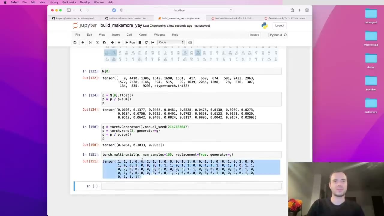 29:31
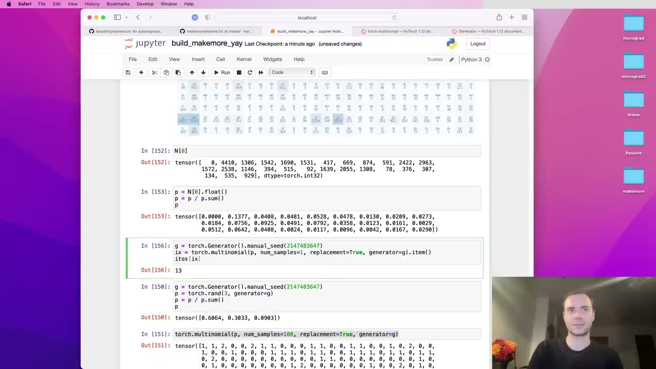 30:44
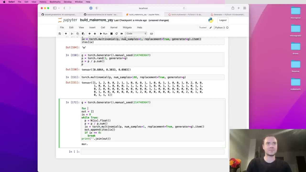 33:56
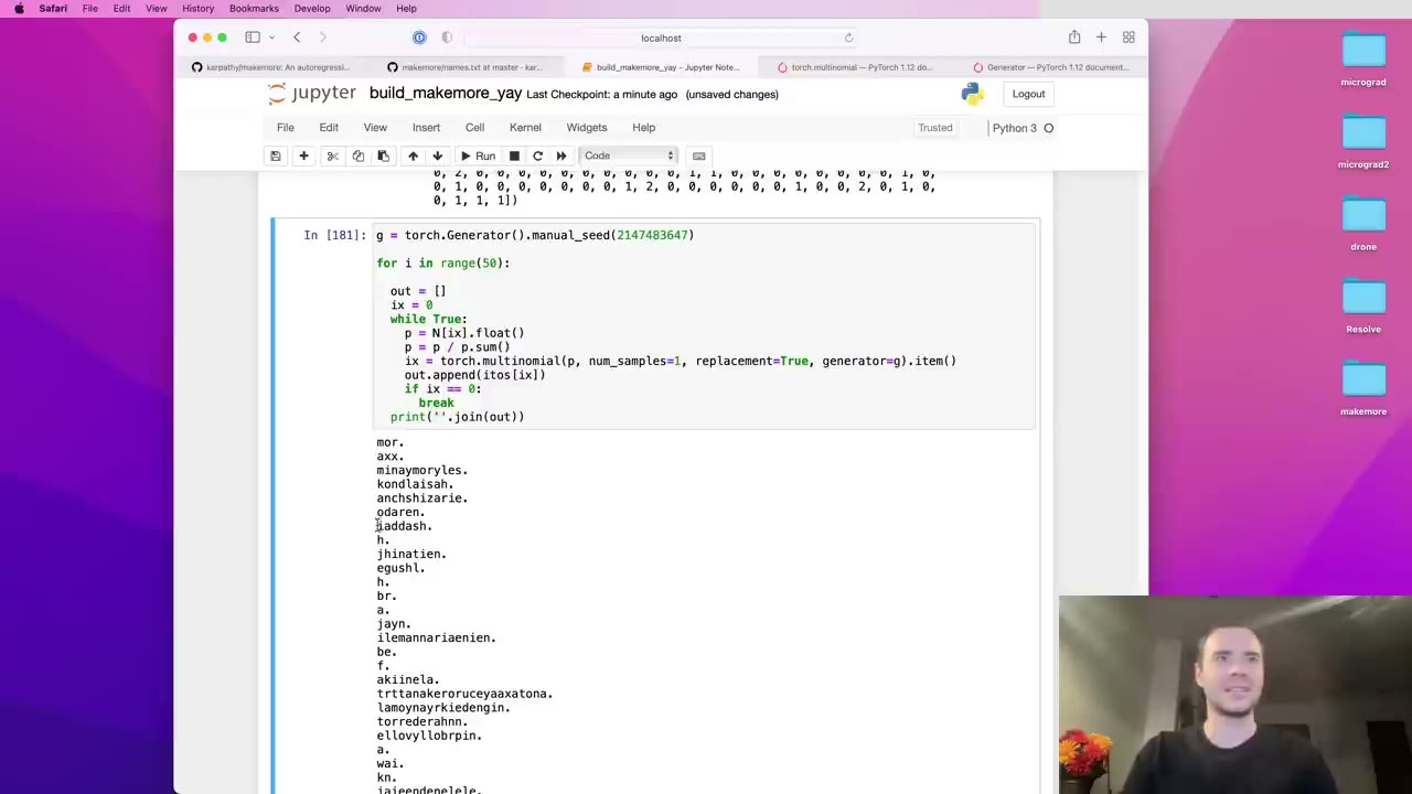 34:57
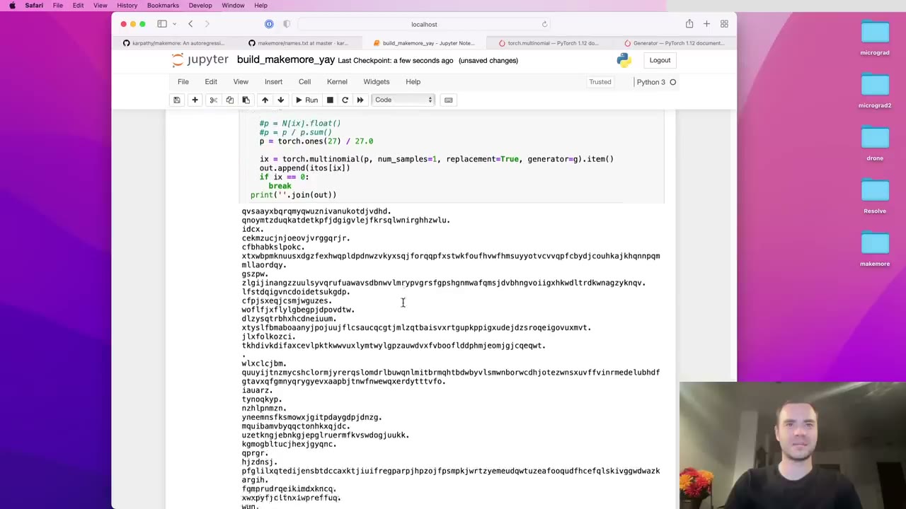 35:54
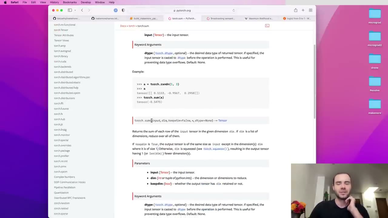 38:37
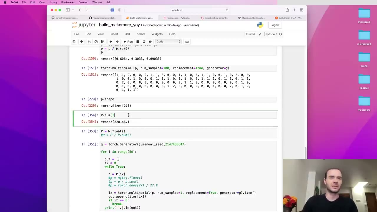 39:26
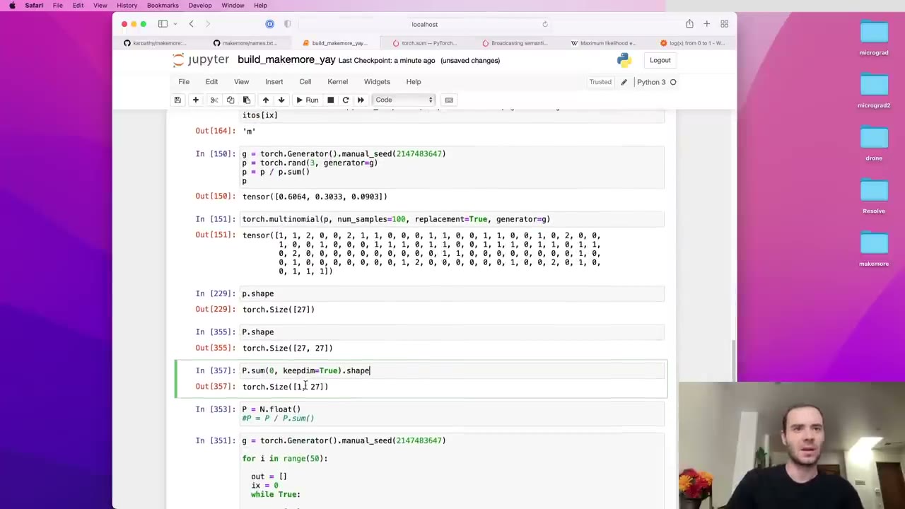 40:15
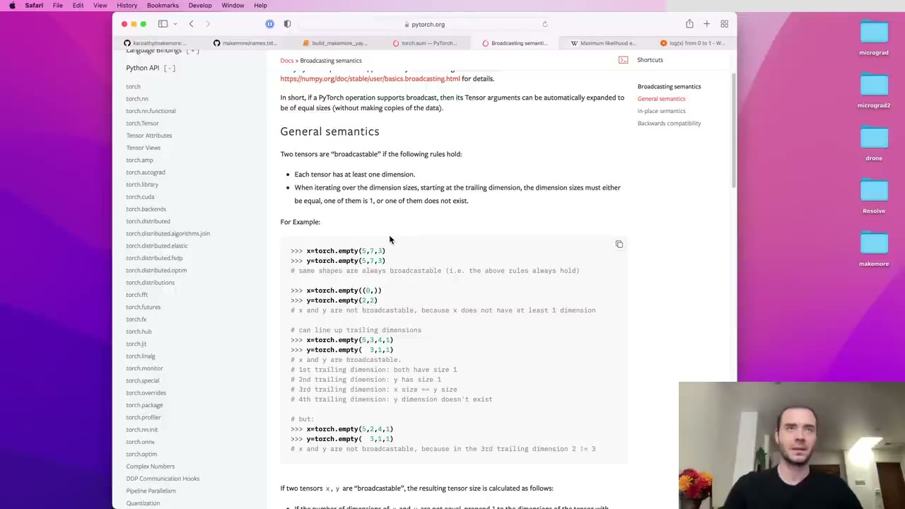 42:23
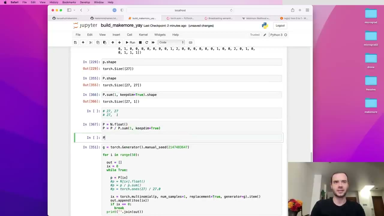 44:00
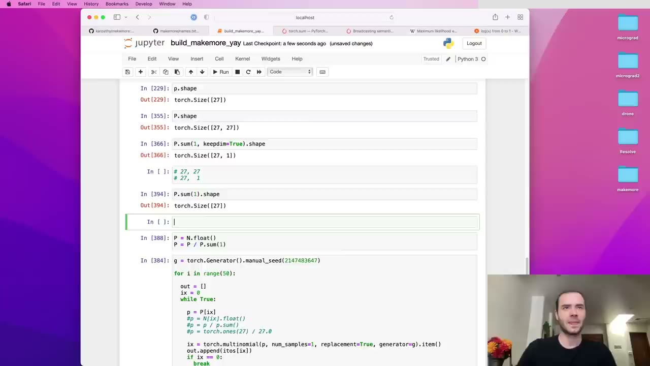 45:51
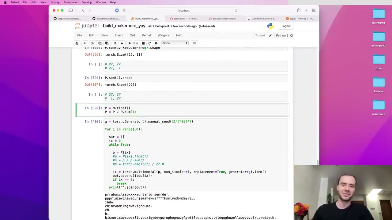 47:13
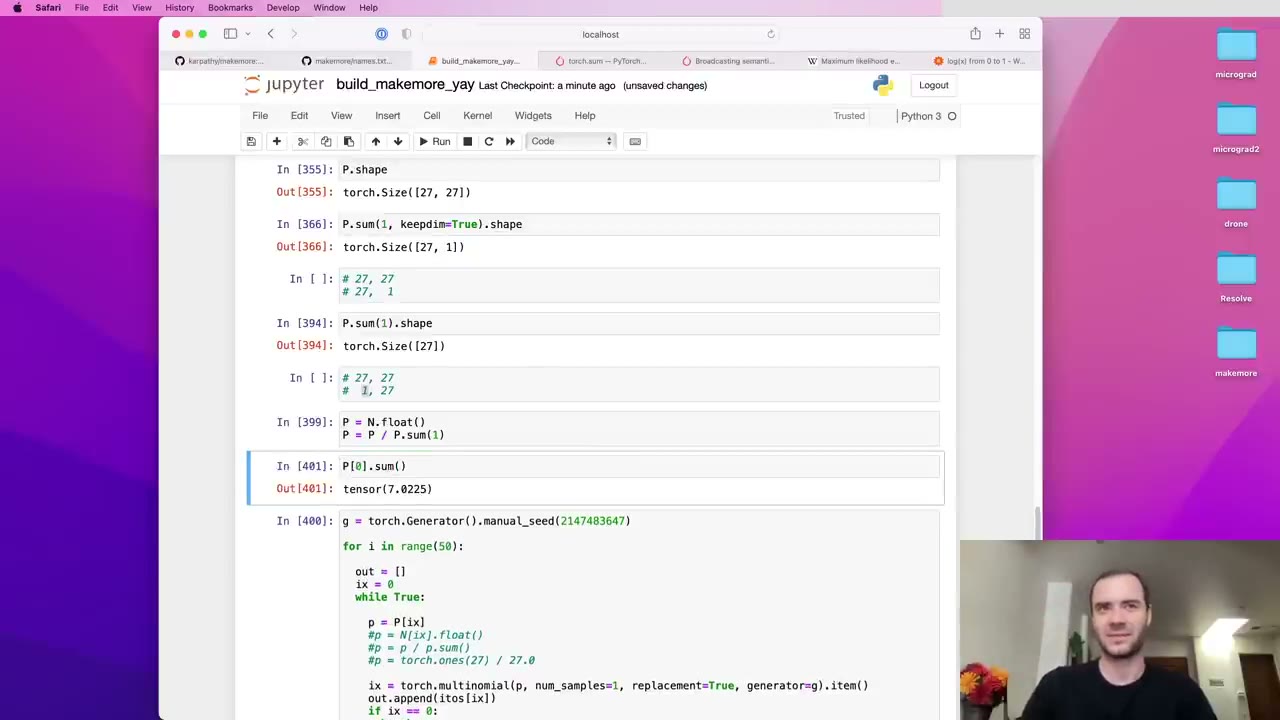 48:17
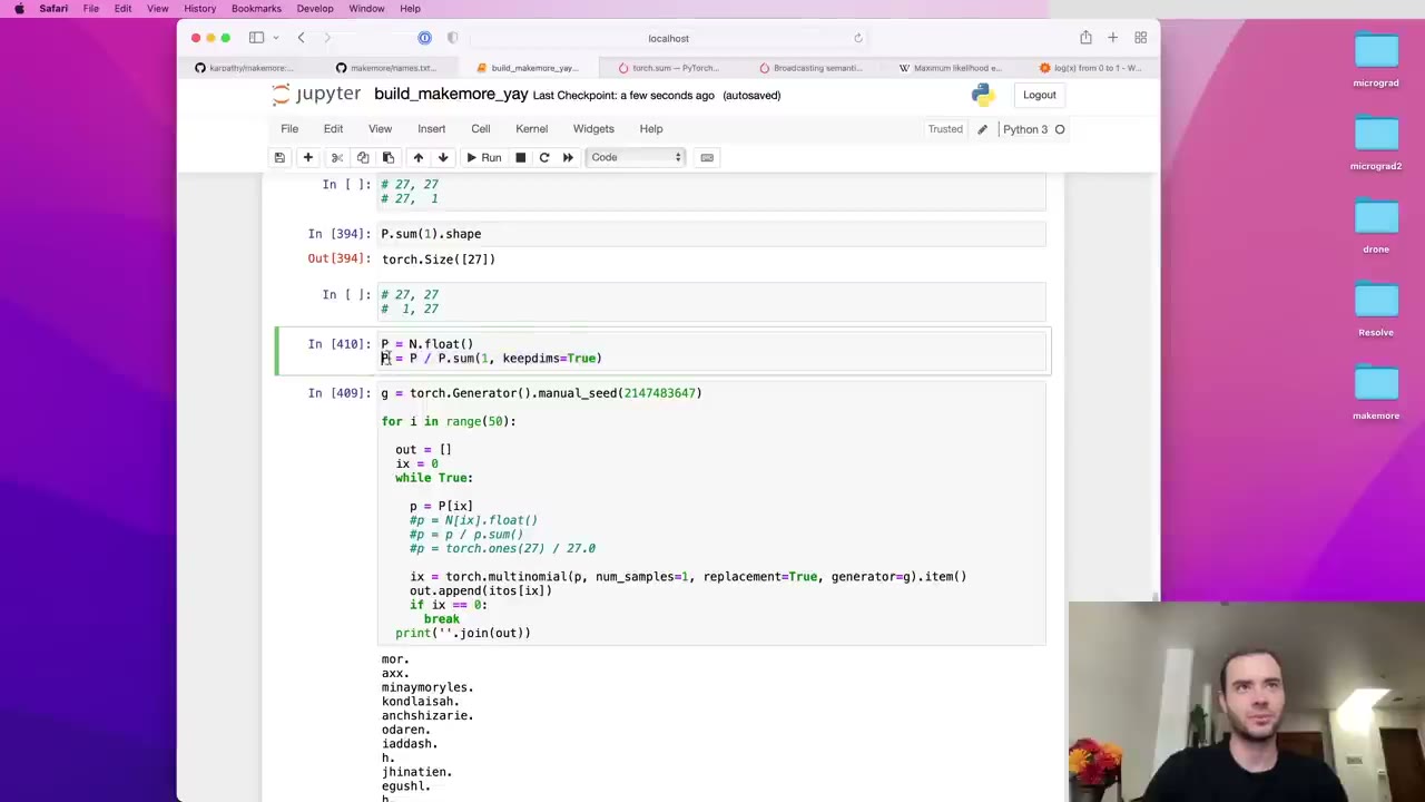 49:53
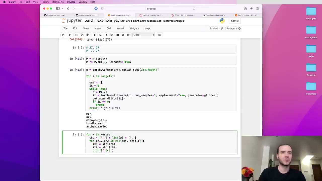 51:28
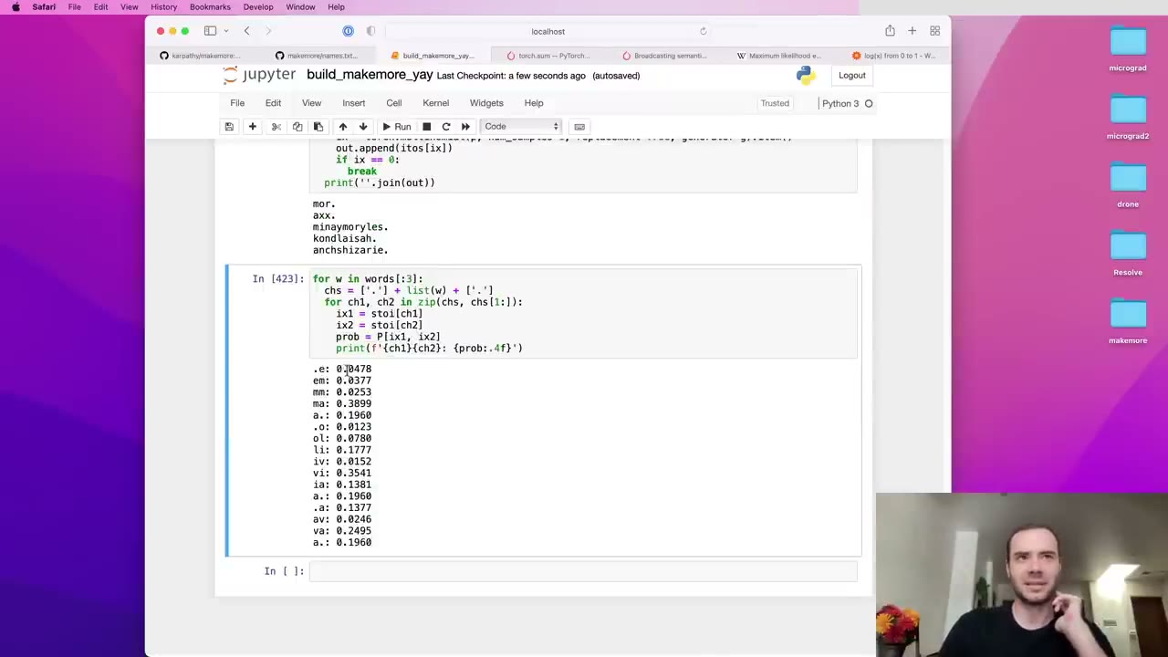 52:11
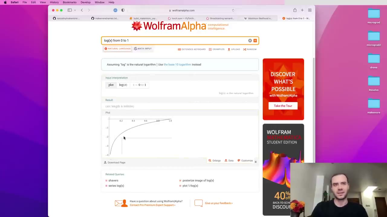 54:20
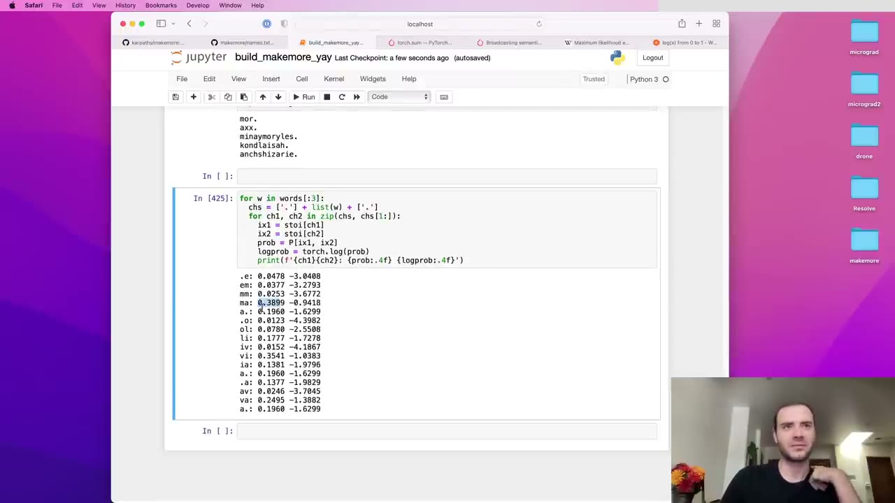 55:00
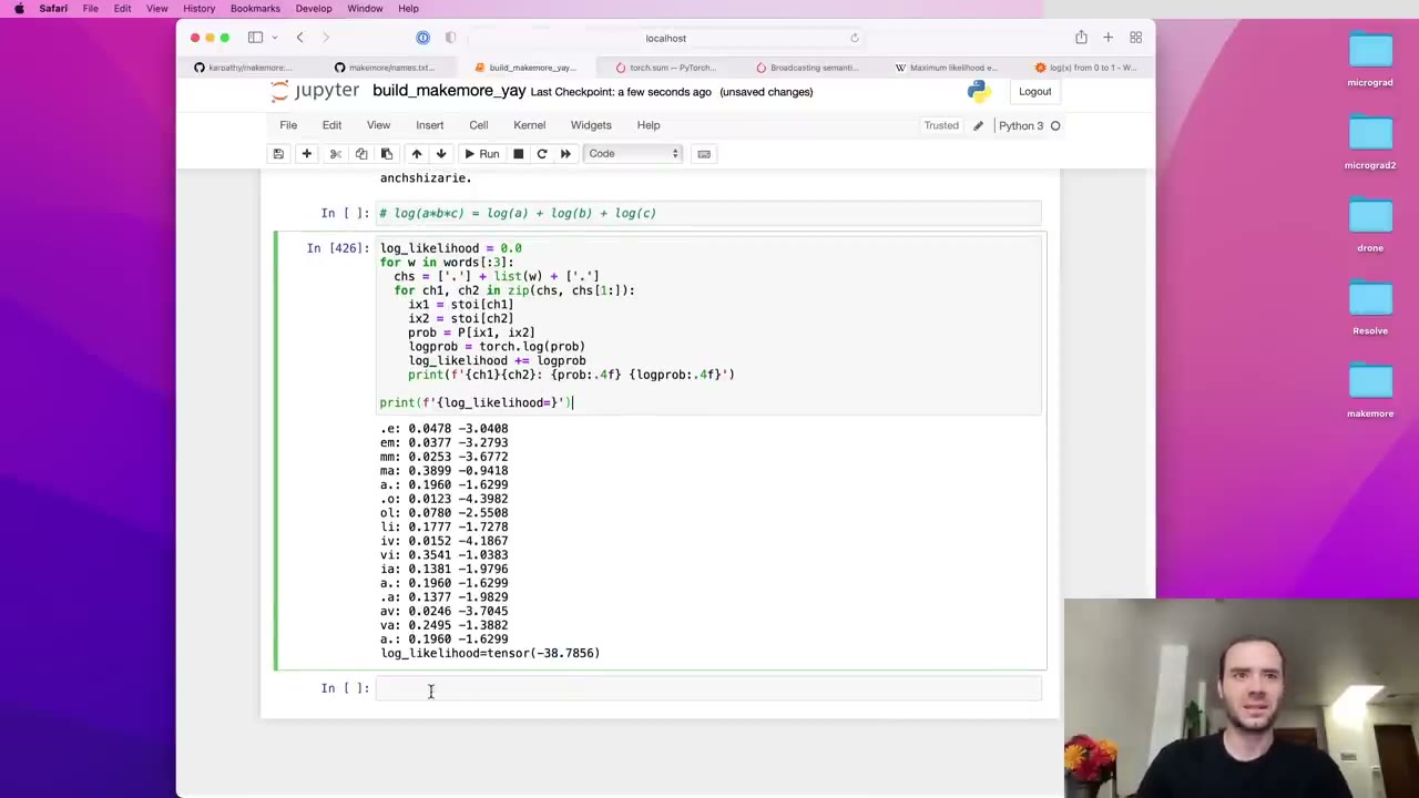 56:23
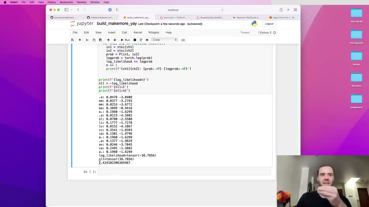 58:05
 59:13
 1:00:25
 1:00:38
 1:01:03
 1:02:44
 1:05:48
 1:07:19
 1:08:37
 1:08:59
 1:11:11
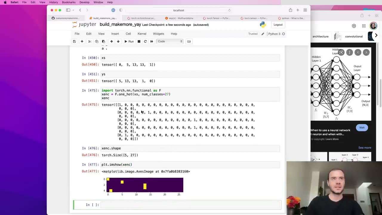 1:12:15
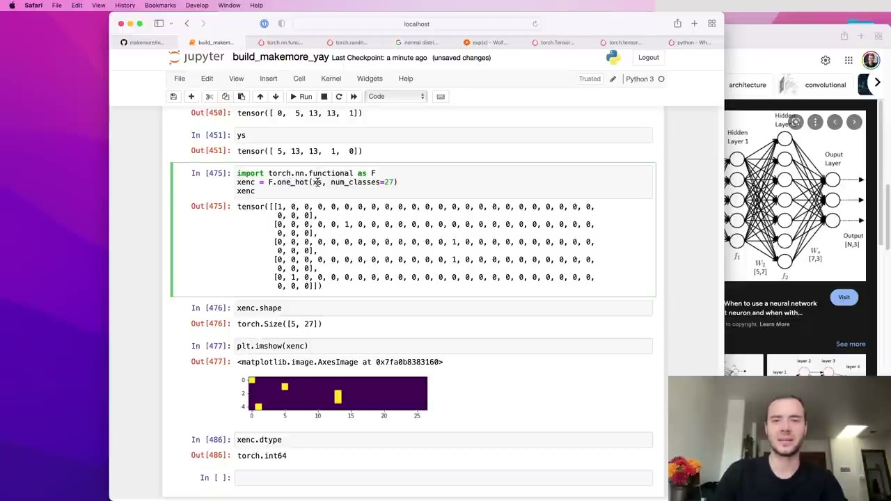 1:13:17
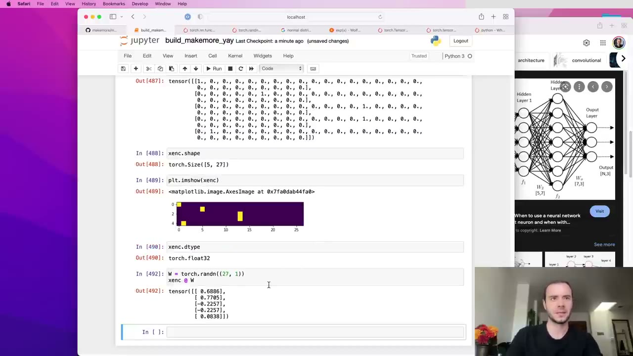 1:15:19
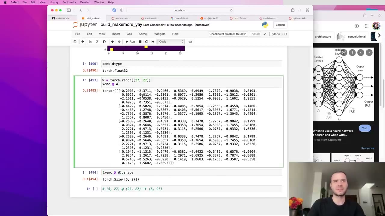 1:17:04
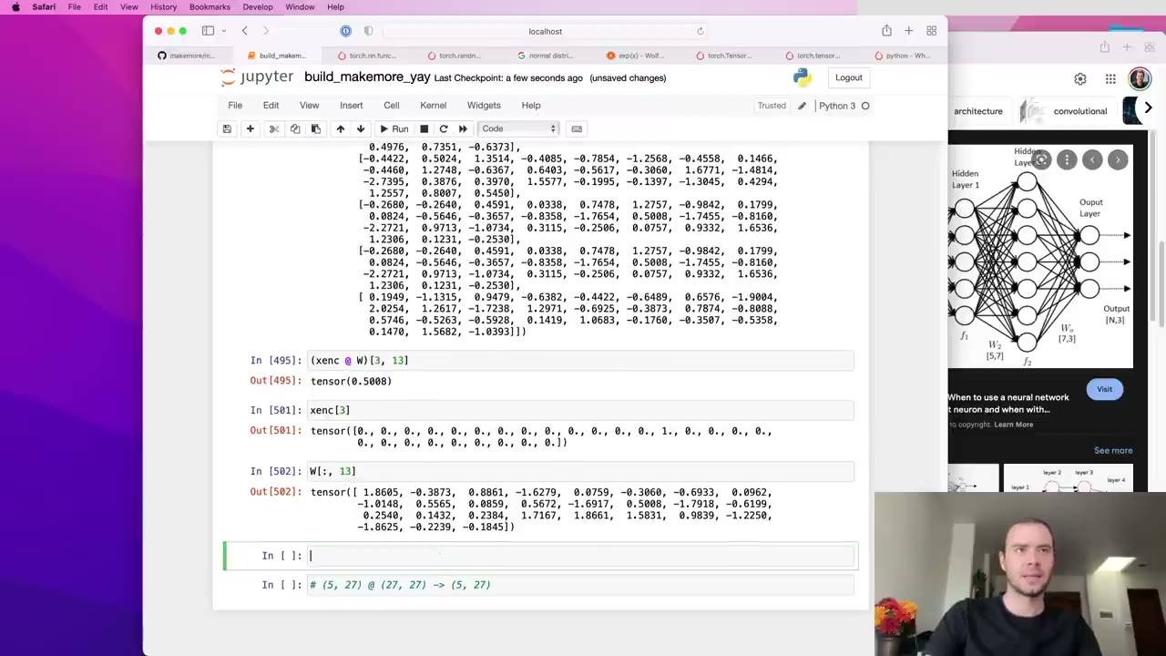 1:18:17
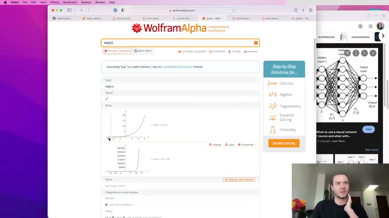 1:21:06
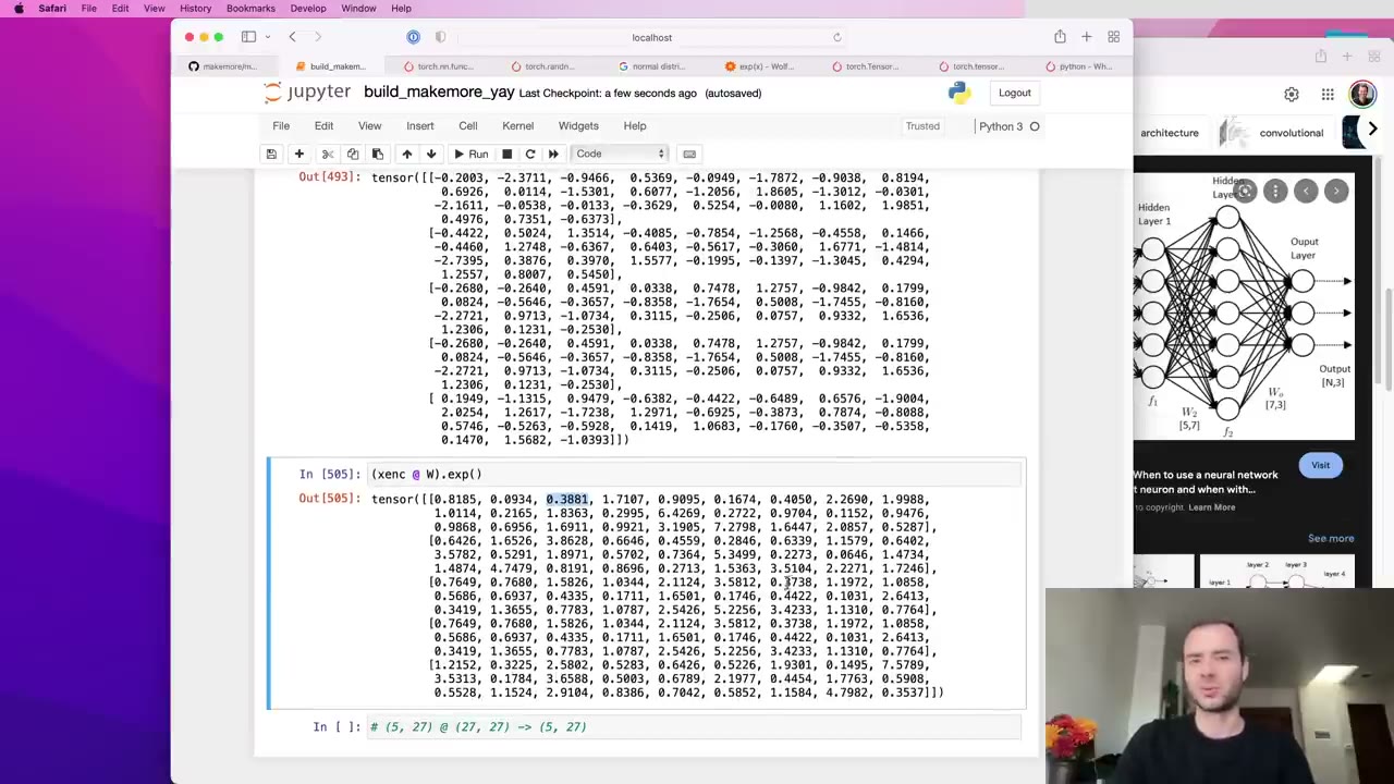 1:22:07
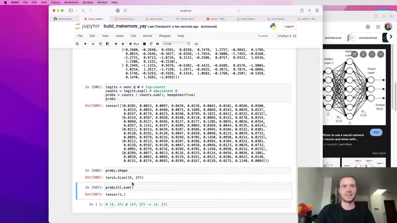 1:24:27
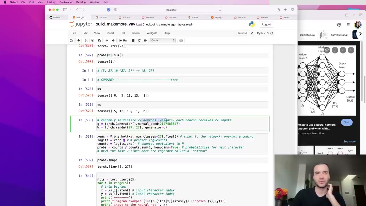 1:26:41
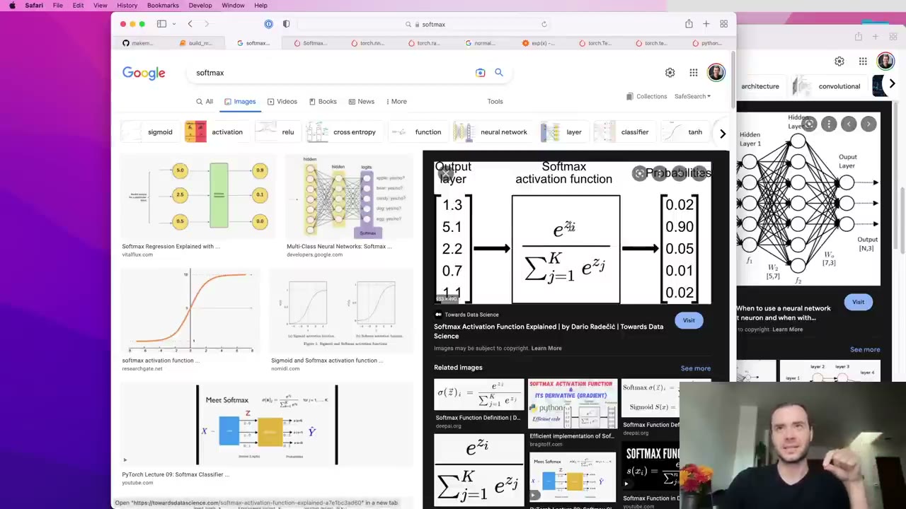 1:27:36
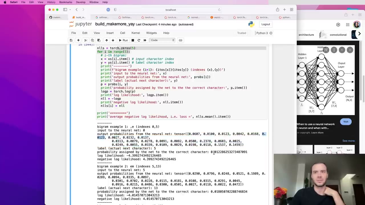 1:30:01
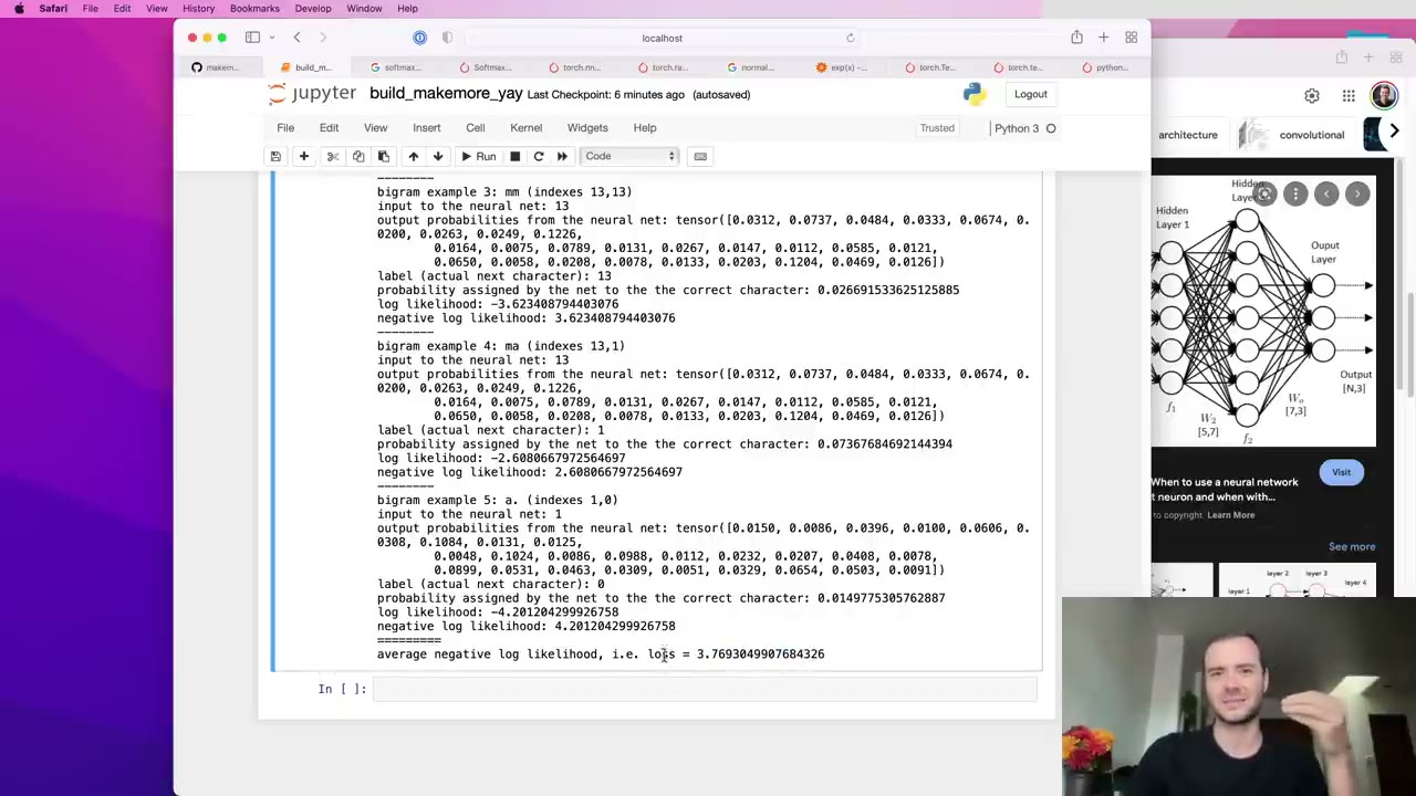 1:31:35
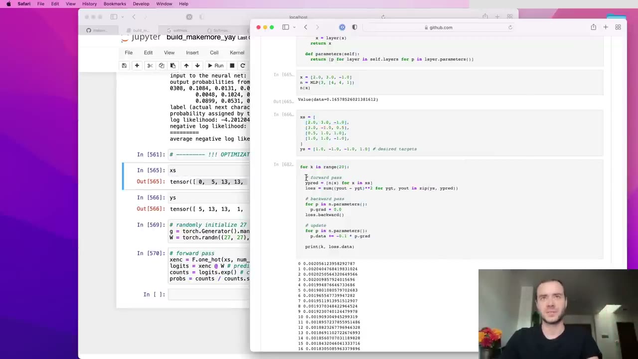 1:33:53
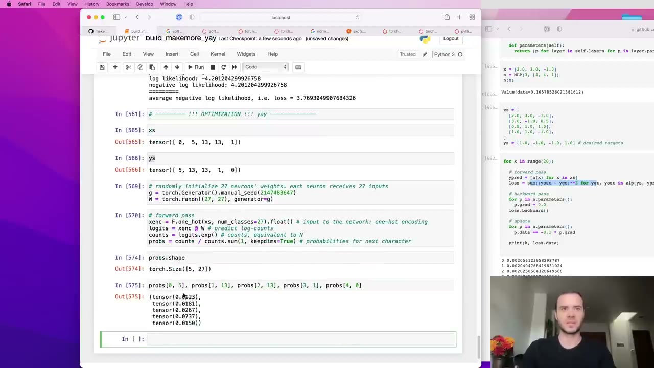 1:36:52
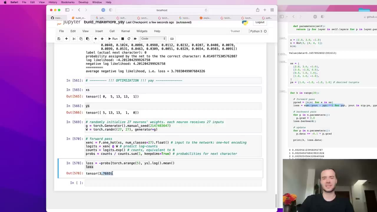 1:38:21
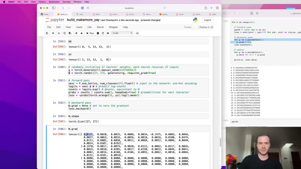 1:40:46
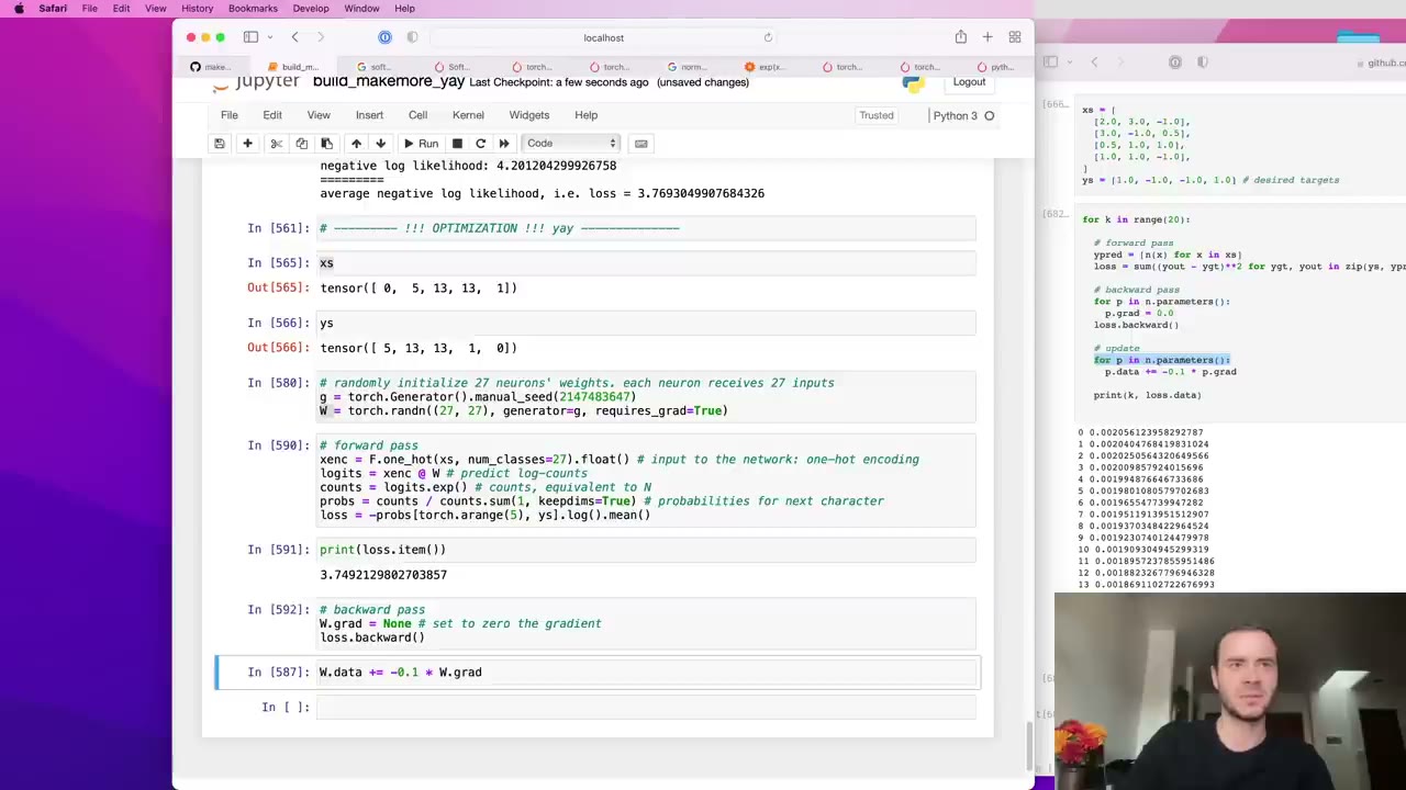 1:42:30
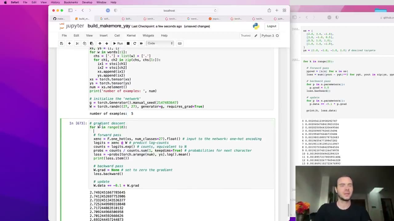 1:43:20
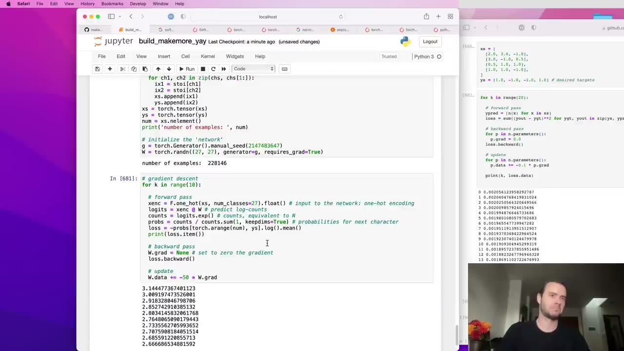 1:44:20
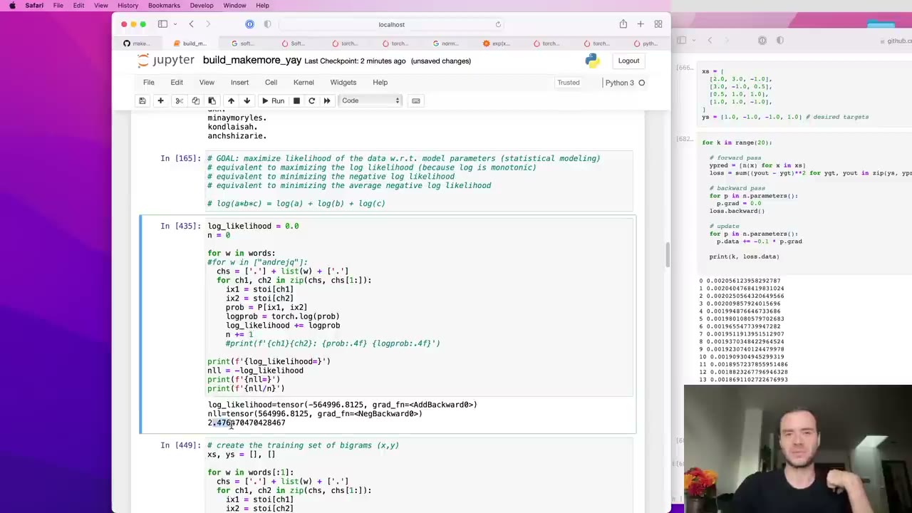 1:45:00
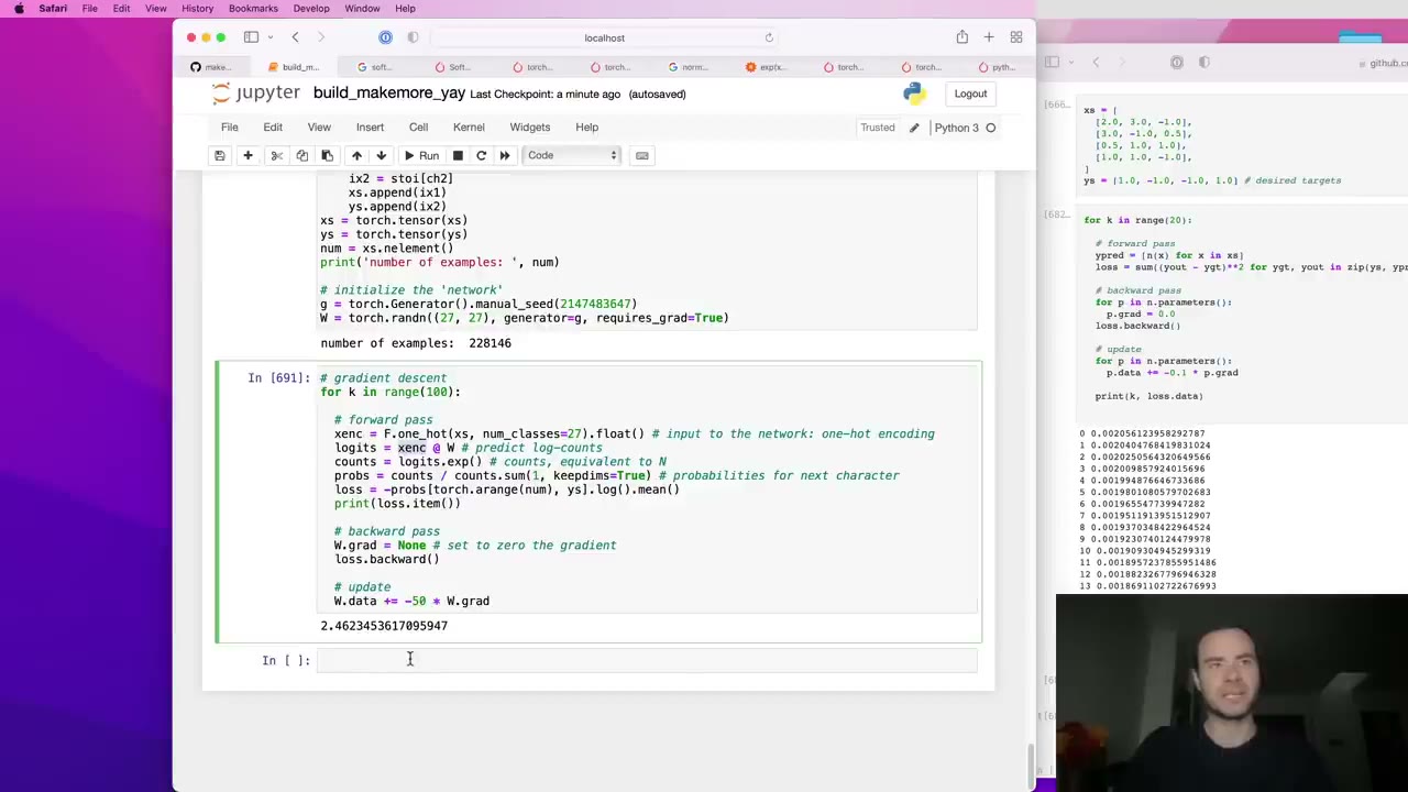 1:48:10
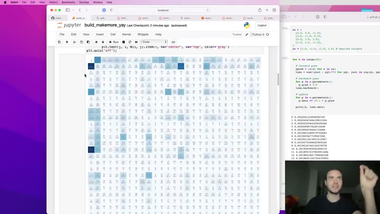 1:48:50
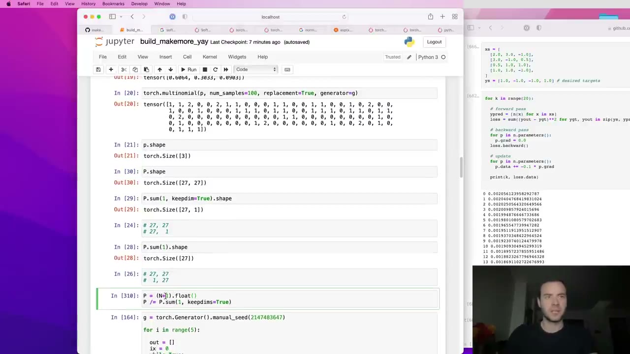 1:50:20
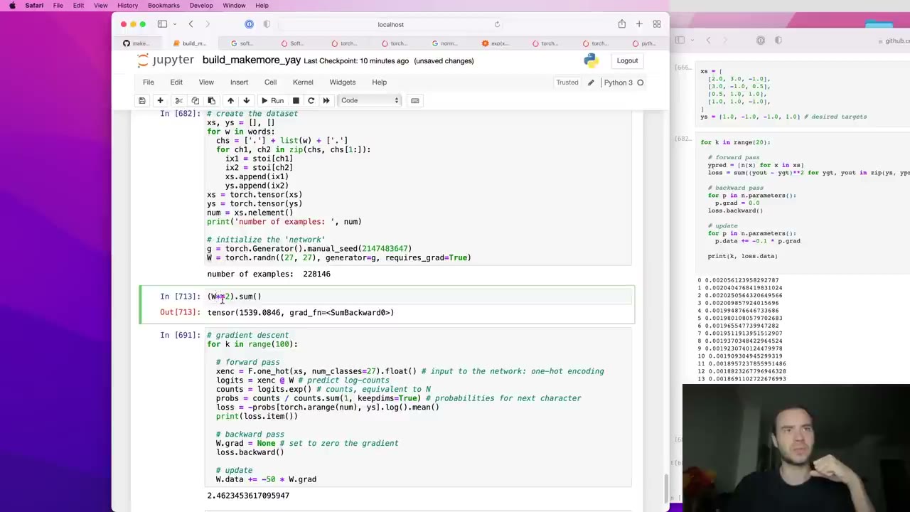 1:52:32
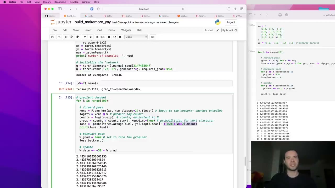 1:53:43
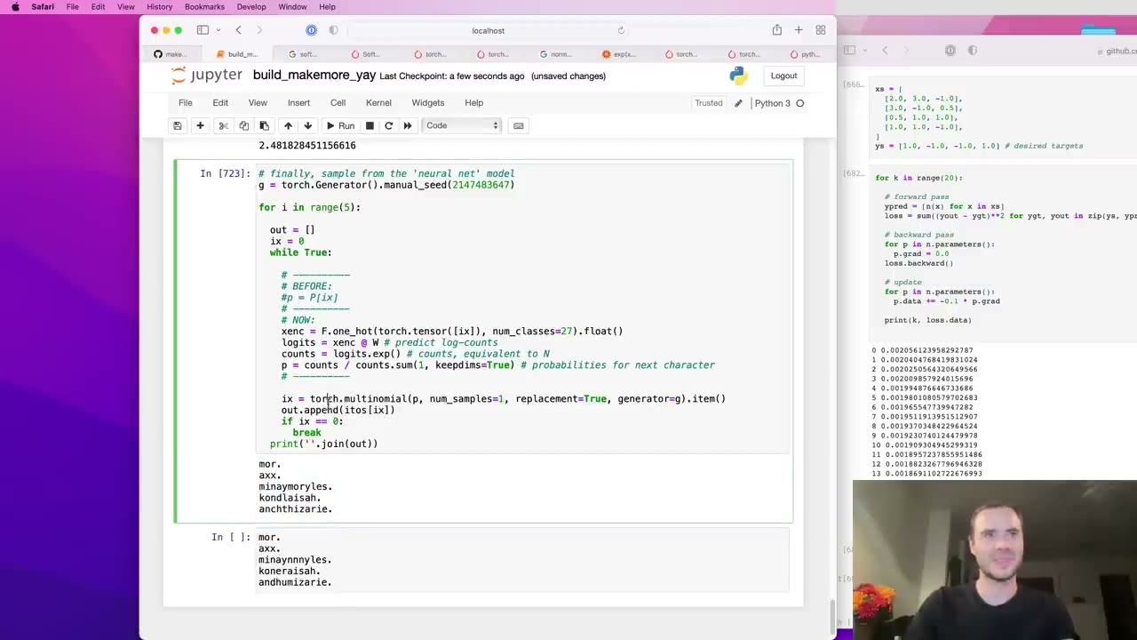 1:55:50
Watch the video (118 min)
Watch the original video on YouTube
Lecture 2 of Andrej Karpathy’s Neural Networks: Zero to Hero series moves from scalar autograd to language modeling. Where Lecture 1 built micrograd, this one starts makemore, a character-level model that learns from about 32,000 names and generates new name-like strings. The whole lecture stays with the simplest possible version, a bigram model that predicts each character from the one before it, and builds it twice. First by plain counting, which yields a table of probabilities, a sampler and a loss. Then as a one-layer neural network in PyTorch, trained by gradient descent, which ends up at essentially the same table. The point of the second build is not a better model but a framework that scales: the softmax, the negative log likelihood loss and the training loop introduced here stay the same all the way up to transformers. Along the way you get a careful lesson in tensor broadcasting that is worth the price of admission on its own. The next step, Lecture 3, gives the model more than one character of context.
Key takeaways
- One name holds several training examples (4:39). “isabella” says which letter tends to start a name, which letters follow which, and that the name ends after the last “a”. Padding each word with a start/end token captures all of it.
- A bigram model is just a normalized count table (23:31). Rows are the current character, columns the next one; normalize each row and you can sample names by walking it.
- Broadcasting can be silently wrong (46:42). Dropping
keepdim=Truestill runs but normalizes columns instead of rows. Check shapes and sums. - Average negative log likelihood is the loss (57:42). Multiply the probabilities the model gives the real data, take logs, negate and average: lower is better, zero is perfect. The counted model scores about 2.45.
- Logits plus softmax turn any layer into a probability model (1:27:14). Read the outputs as log counts, exponentiate, normalize each row.
- Gradient descent recovers the counting solution (1:45:15). With the same information in, the one-layer net reaches the same loss, and
W.exp()plays the role of the count table. - Smoothing and regularization are the same lever (1:53:34). Adding fake counts in the table world corresponds to pulling
Wtoward zero in the network world. - Only the forward pass will change from here on (1:46:48). Logits, softmax, loss and update stay fixed while the network grows toward a transformer.
Chapter notes
0:02 – 5:42 What makemore is, and the names dataset
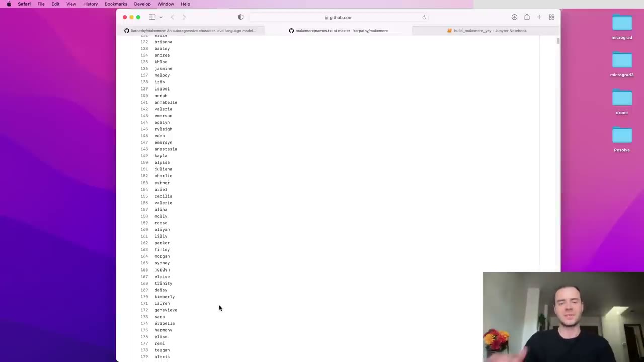
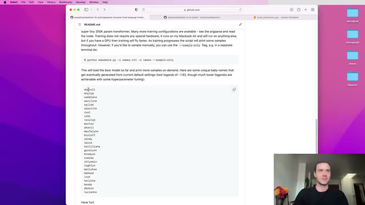
makemore, like micrograd, is a repository on Karpathy’s GitHub that he rebuilds from a blank notebook. Its job is in the name: give it a dataset and it makes more things like it. The example dataset, names.txt, holds about 32,000 names that he says he found on a government website (0:32). After training, the model invents strings that sound like names but aren’t in the list.
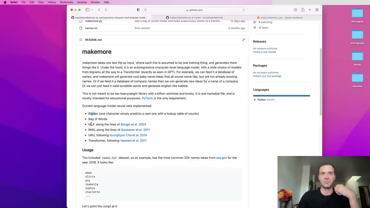
Under the hood it is a character-level language model (1:35): each line is one example, each example is a sequence of characters, and the model’s task is to predict the next character. Karpathy lays out the plan for the series (2:05): bigram and bag-of-words models, multilayer perceptrons, recurrent networks, and finally a transformer he calls the equivalent of GPT-2, all at the character level. He also floats moving to words and to image models later (2:36).
Our note: as published, the series stayed with text. The later lectures build GPT, a tokenizer and a GPT-2 reproduction rather than image models.
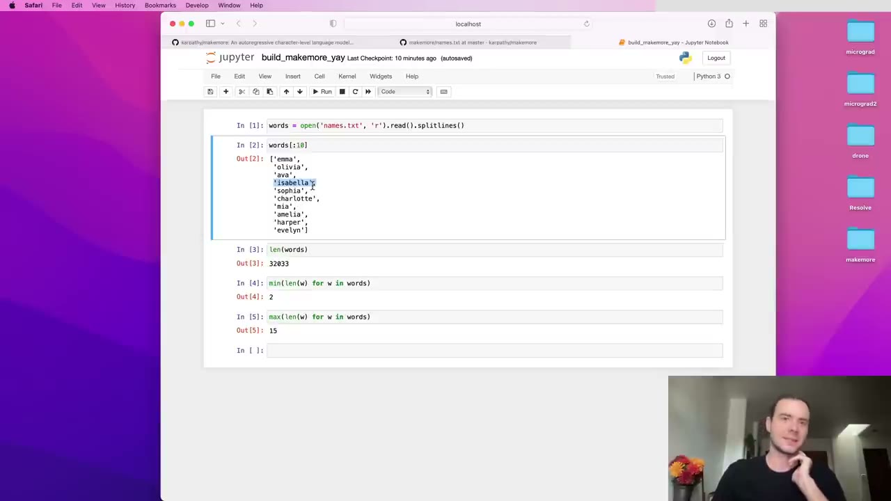
The first cell reads the file and calls splitlines() to get a Python list of names (3:07). The list starts emma, olivia, ava, which makes Karpathy suspect it is sorted by frequency. The shortest name has 2 characters and the longest 15 (4:09).
Then the key observation: a single word is several examples packed together (4:39). It tells you which character is likely to come first, which is likely after “i”, which after “is”, and so on, plus one easy-to-miss fact: after the full word, the name ends (5:12).
5:42 – 12:29 Bigrams, counted in a dictionary
A bigram model looks at only two characters at a time: given one, predict the next (5:42). It ignores everything earlier in the word, which makes it weak, but it is the right first step.
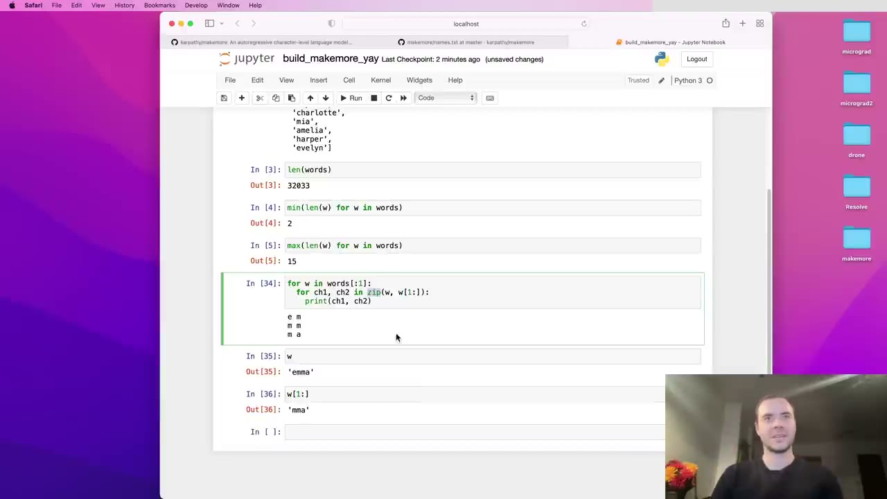
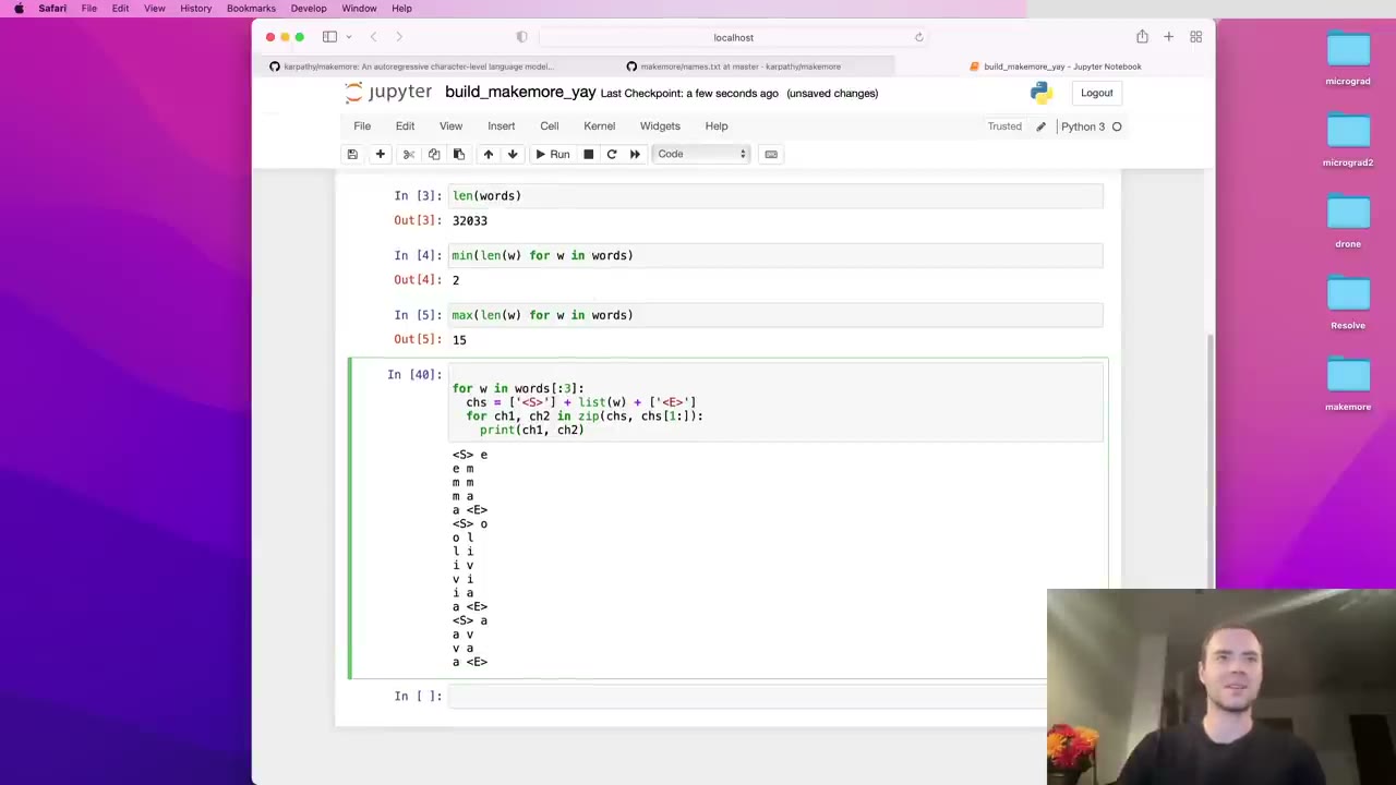
To list consecutive pairs, Karpathy uses zip(w, w[1:]) (6:44). Zipping a string with itself shifted by one pairs each character with its successor, and zip stops when the shorter input runs out (7:15). To keep the start and end information, he wraps each word as a list with a special <S> token in front and <E> behind (8:17).
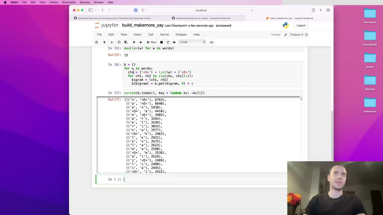
Counting is a dictionary keyed by the pair, updated with b.get(bigram, 0) + 1 so unseen pairs start at zero (9:49). On the first three names, “a” followed by <E> already shows up three times, since emma, olivia and ava all end in “a” (10:20). Over the whole dataset he sorts b.items() by count with a lambda key (11:27): rare pairs appear once, while “n” ending a name and “a” followed by “n” are among the most frequent (12:29).
12:29 – 18:10 Moving the counts into a PyTorch tensor
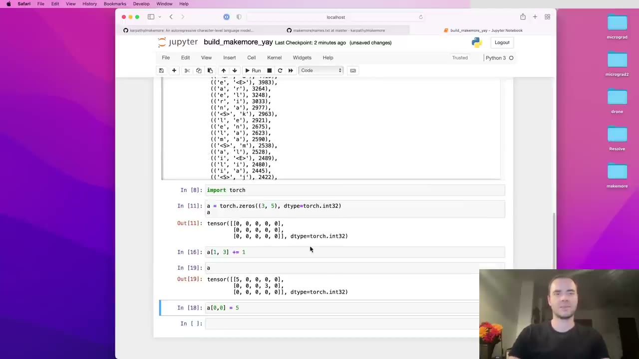
A two-dimensional array is far more convenient than a dictionary: rows for the first character, columns for the second (13:00). Karpathy introduces torch.tensor arrays here. torch.zeros defaults to float32, so for counts he asks for dtype=torch.int32 (13:32), then shows basic indexing and in-place increments on a small 3 by 5 example (14:35).
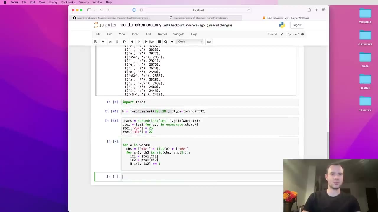
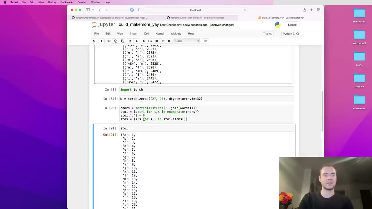
The real table needs 26 letters plus two special tokens, so 28 by 28 (15:08). Indexing a tensor needs integers, so he builds a lookup: join all names into one string, take its set of characters, and sort it (16:09). stoi maps “a” to 0 through “z” to 25, with <S> and <E> appended as 26 and 27 (17:10). The counting loop then becomes N[ix1, ix2] += 1 (17:40).
18:10 – 24:02 Visualizing the table, then one ‘.’ token
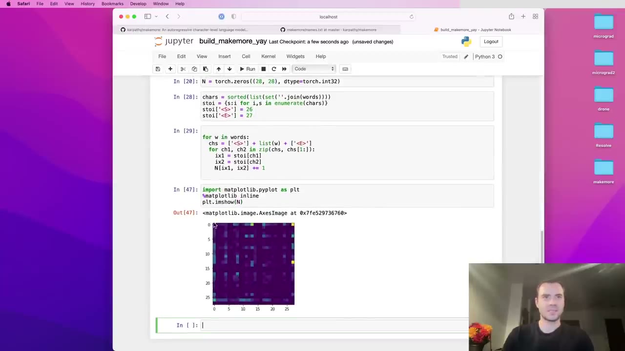
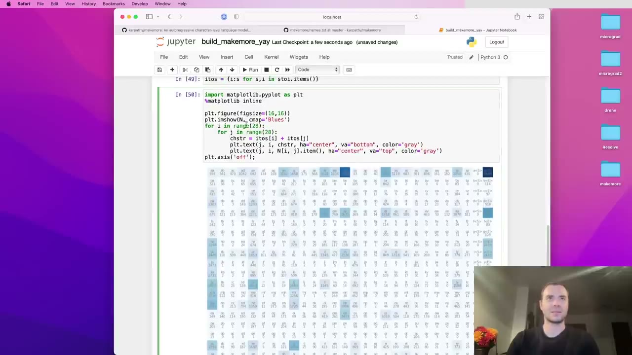
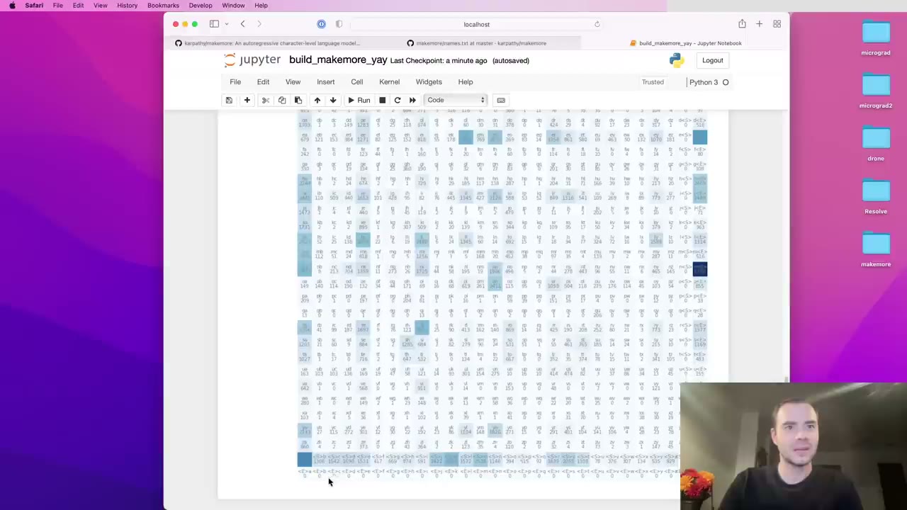
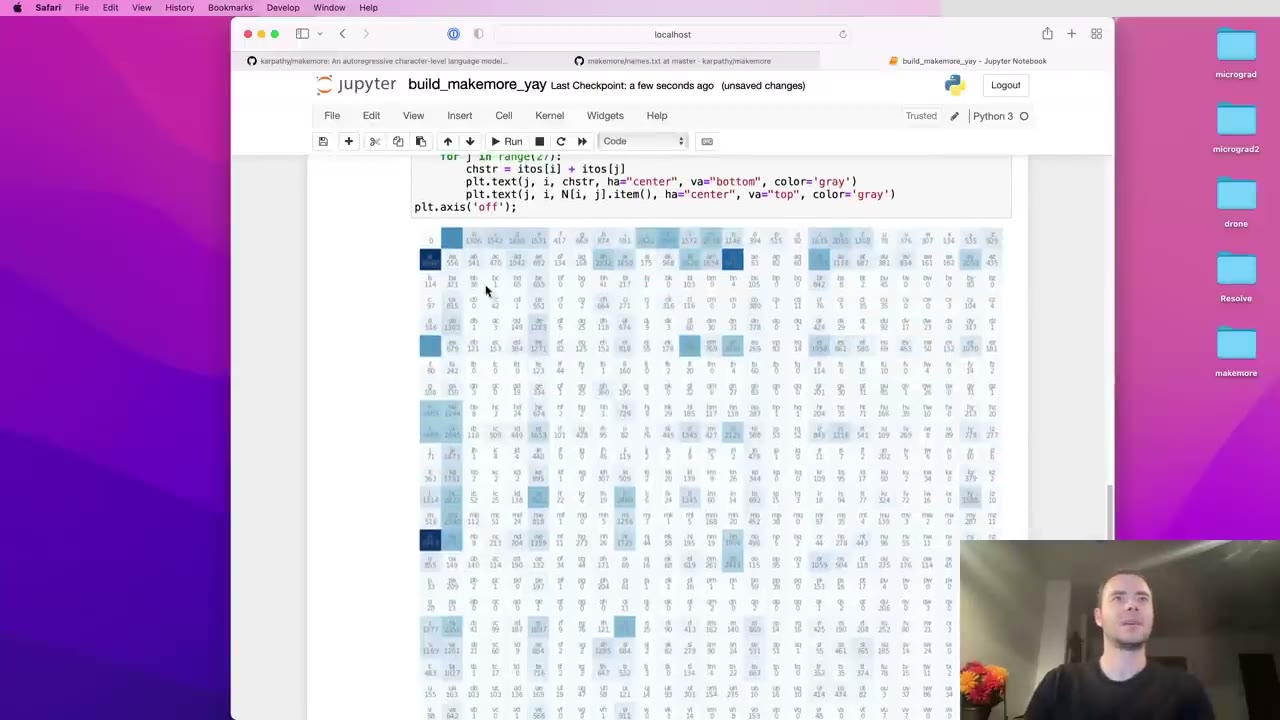
Printed raw, the array is unreadable, so Karpathy plots it with Matplotlib’s imshow (18:10) and writes each cell’s bigram and count on top, using the inverse mapping itos (18:41). A side lesson: indexing a tensor returns a tensor, so .item() is needed to pull out a plain Python number (20:17).
The plot exposes waste (20:49). The <E> row is all zeros because the end token never starts a bigram, and the <S> column is all zeros because the start token never follows anything (21:19). The fix is a single special token, written as “.”, that serves as both start and end (21:50). It takes index 0 and the letters shift to 1 through 26, giving a 27 by 27 table (22:21).
The new table reads cleanly (23:31). The first row counts how often each letter starts a name, the first column how often each letter ends one, the “.” to “.” cell is zero because there are no empty names, and everything in between is letter-to-letter structure. That table is everything needed to sample.
24:02 – 36:20 Sampling names from the counts
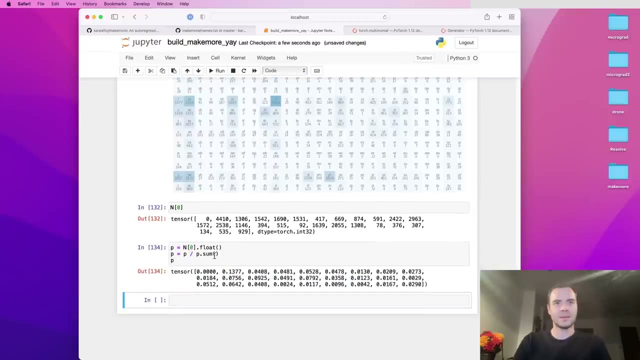
Sampling starts at the “.” token, so the first character comes from row 0 (24:02). N[0] gives that row as a vector of 27 counts. Convert it to float and divide by its sum to get probabilities that add up to one (25:35).
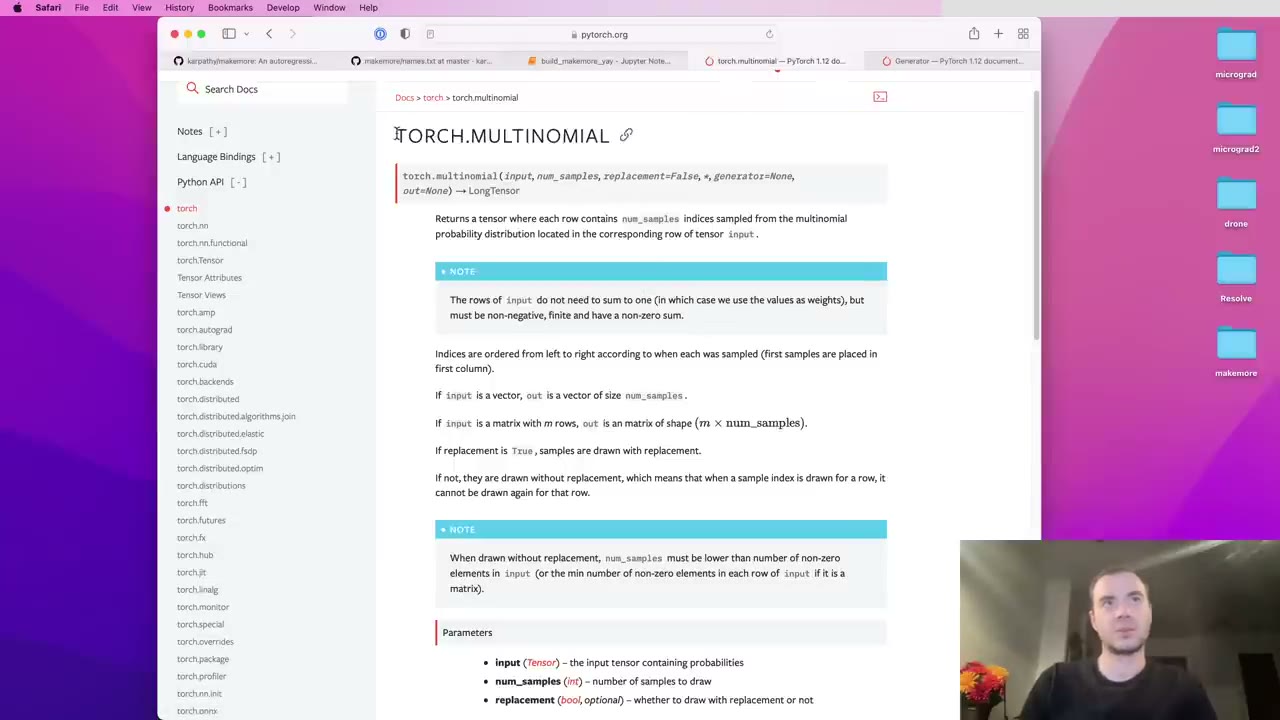
To draw from it, Karpathy uses torch.multinomial: give it probabilities and it returns sampled integer indices (26:36). A seeded torch.Generator makes the results reproducible, so viewers get the same samples he does (27:07). He demonstrates on a random three-element distribution, noting that replacement=True must be passed explicitly because it defaults to False (28:09), and checks that sample frequencies roughly match the probabilities (29:10).
Back on the real row, the first draw is index 13, the letter “m” (30:12), which plausibly starts about 2,500 of the 32,000 names (30:43). The next character comes from the “m” row, and so on. Written as a loop (31:46): start at index 0, take the current row, normalize, sample, stop when the sample is 0 again. The first generated name is “mor.” (33:05).
Run in a loop, most names look bad (34:15). Karpathy explains why from the model’s point of view: after an “h” it has no idea whether that “h” was the first letter, so ending the name right there seems reasonable. To confirm the model is still doing something, he swaps in a uniform distribution, torch.ones(27) / 27 (35:17). That untrained baseline is pure garbage, so the bigram samples are clearly more name-like; the bigram model is simply very weak (35:49).
36:20 – 44:06 Normalizing every row at once with torch.sum
Re-normalizing a row on every step of the loop is wasteful, so Karpathy builds a matrix P of probabilities up front (36:20). He is also open about the second motive: practice with tensor manipulation and broadcasting, which will be essential when the series reaches transformers (37:21).
P.sum() with no arguments adds up the whole matrix, which is not what we want (37:53). The docs for torch.sum show the dim argument and keepdim (38:23). Summing over dimension 0 with keepdim gives a 1 by 27 row of column totals (39:27); without keepdim the size-1 dimension is squeezed away, leaving a plain vector of 27 (39:57). Summing over dimension 1 gives the 27 by 1 column of row totals that we actually want (40:31). In this particular table the two sets of totals happen to be identical (41:01).
Our note: that coincidence has a reason. In a padded word every letter has exactly one bigram leading in and one leading out, and each word contributes one “.” at the start and one at the end, so each character’s row total equals its column total.
Can a 27 by 27 tensor be divided by a 27 by 1 tensor? Broadcasting rules decide (42:03). Align the shapes on the right, then walk leftward: each pair of sizes must be equal, or one of them must be 1, or one must be missing (42:33). Here that holds, so PyTorch stretches the column across all 27 columns and divides element-wise (43:05), normalizing every row (43:36). The check is that row 0 now sums to one and sampling from P gives the same names as before.
44:06 – 50:17 The keepdim bug
Karpathy urges viewers to read the broadcasting rules and to treat this with respect (44:06), then shows why. Remove keepdim=True and the row totals come back as a vector of 27, with the same numbers (45:09). Run the rules again: the shapes are still broadcastable (45:40), because the missing dimension gets filled in as 1 (46:10). The division runs, and the result is garbage (46:42).
He pauses for viewers to work it out, then explains (47:12). The new dimension is added on the left, so the vector of 27 becomes a 1 by 27 row. That row is copied down 27 times (47:43), and each column ends up divided by totals meant for rows. Row 0 of the result sums to 7, while it is the columns that now sum to one (48:13).
The lesson (49:15): check your shapes, know which direction a broadcast goes, and expect these bugs to be hard to find because nothing crashes. He finishes with an efficiency touch, using the in-place P /= ... so no new tensor is allocated (49:46).
50:17 – 1:00:17 Scoring the model: from likelihood to negative log likelihood
The entries of P are the model’s parameters, found by counting (50:17). Now Karpathy wants one number that says how good they are on the training set, a training loss as in micrograd (50:47).
He prints the probability the model assigns to each actual bigram in the first three names (51:48). As a yardstick, uniform guessing over 27 tokens gives about 4% each, so values like 35% or 40% mean the model has learned something (52:19). A perfect model would give probabilities near 1.
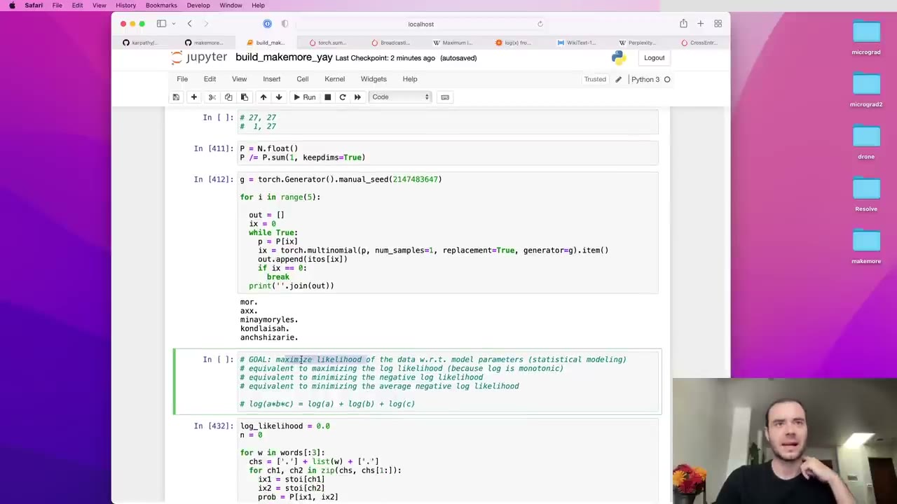
The textbook summary from maximum likelihood estimation is the likelihood, the product of all those probabilities (53:21). Multiplying many numbers below one gives something tiny, so in practice you take logs (53:51). The log is monotonic, 0 at probability 1 and heading to minus infinity as probability falls to 0 (54:21), and the log of a product is the sum of the logs (55:27). The log likelihood of the three names comes to about −38 (56:11).
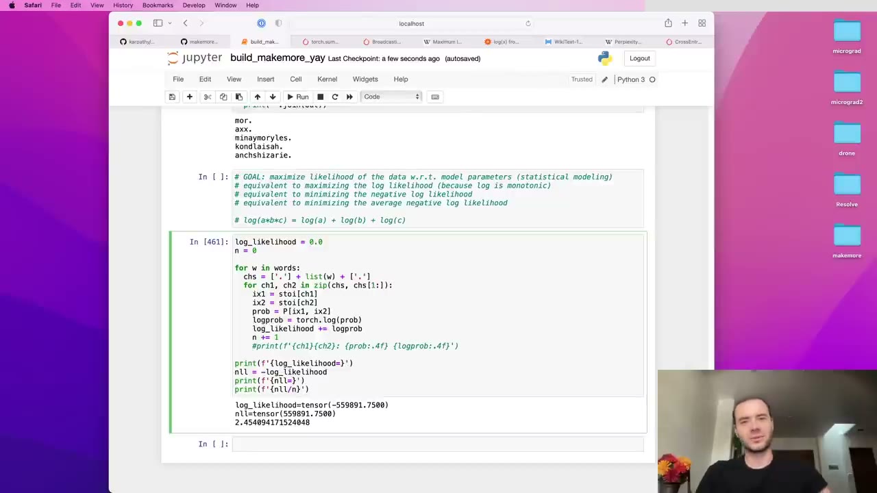
A loss should go down when things get better, so negate it: the negative log likelihood is zero at best and grows as predictions get worse (56:41). Divide by the number of bigrams for an average (57:12), and the three names score about 2.4 (57:42).
| Step | Quantity | Better when |
|---|---|---|
| Product of probabilities | likelihood | higher |
| Sum of log probabilities | log likelihood | higher (max 0) |
| Negated | negative log likelihood | lower (min 0) |
| Divided by count | average NLL, the loss | lower |
Karpathy summarizes the chain (58:13): maximize likelihood with respect to the parameters, which is the same as maximizing log likelihood, the same as minimizing negative log likelihood, the same as minimizing its average (59:15). He previews the turn the lecture is about to take: these probabilities won’t stay in a table but will be computed by a neural network whose parameters we tune (58:43).
1:00:17 – 1:03:51 Infinite loss and model smoothing
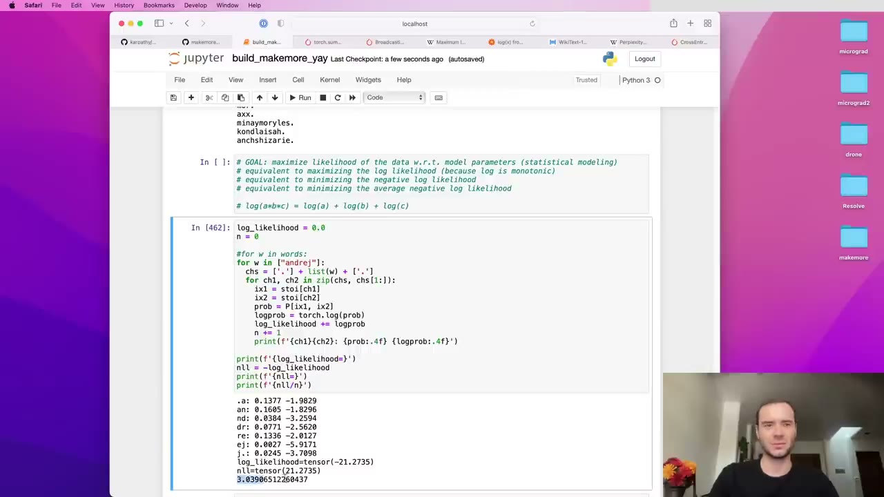
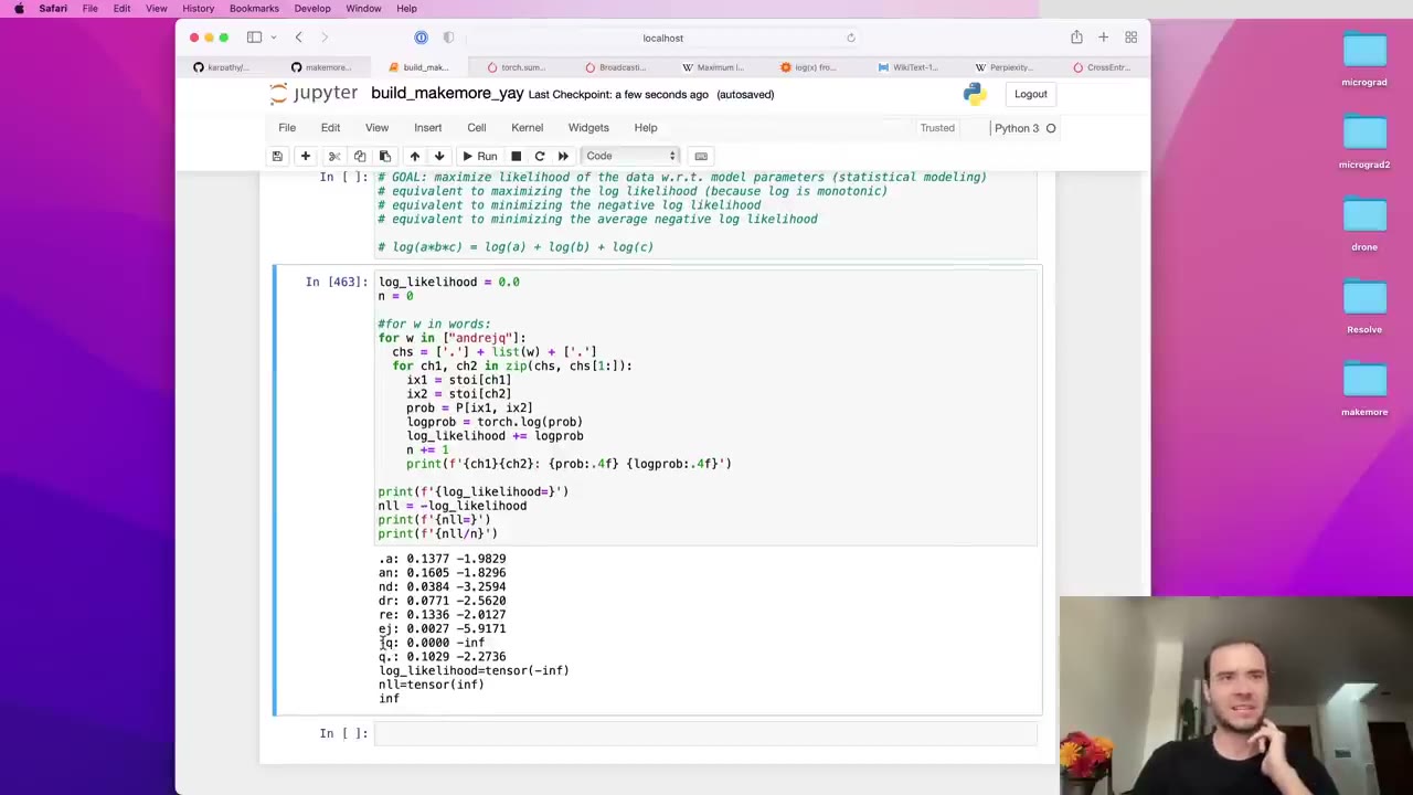
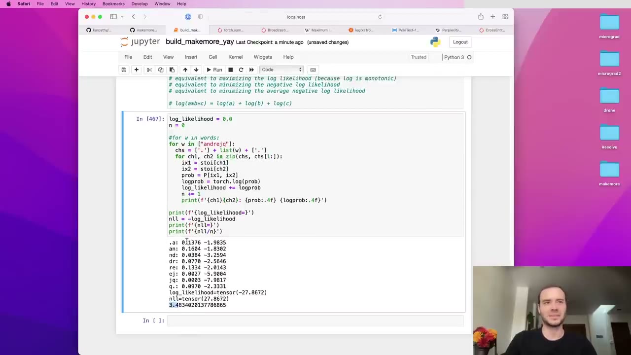
Over the full training set the loss is about 2.45 (1:00:17). The same loop can score any string. Karpathy tries his own name, “andrej”, which averages around 3 per character, largely because “ej” is rare. Then he appends a “q” (1:00:47): “jq” never occurs in the data, its probability is 0, its log is minus infinity, and the loss is infinite (1:01:18).
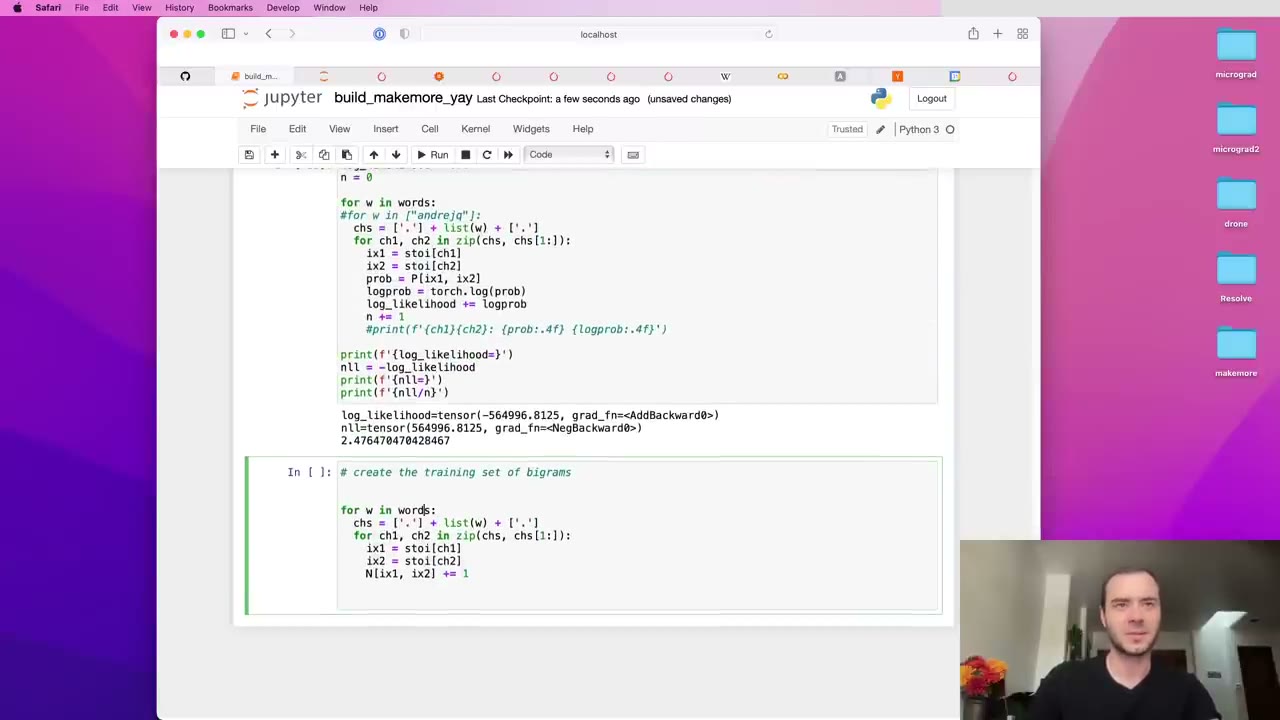
The fix is model smoothing (1:01:49): add fake counts to every cell before normalizing, P = (N+1).float(). The more you add, the more uniform the model; the less, the more peaked (1:02:19). Adding one removes every zero, so “jq” becomes very unlikely rather than impossible.
Our note: add-one smoothing is also known as Laplace smoothing. In the notebook, the smoothed model scores about 2.476 on the training set, slightly worse than unsmoothed, which is the expected trade for never assigning zero probability.
Karpathy then recaps the counting approach (1:02:49): training by counting and normalizing, sampling by walking the rows, evaluating by average negative log likelihood.
1:03:51 – 1:10:02 The same model as a neural network, and its training set
Now the same bigram problem goes into the neural network framework (1:03:51). The network takes one character, passes it through weights W, and outputs a probability distribution over the next character (1:04:21). The label is the actual next character, the loss is the negative log likelihood of that label, and gradient-based optimization tunes W to push the loss down (1:04:53).
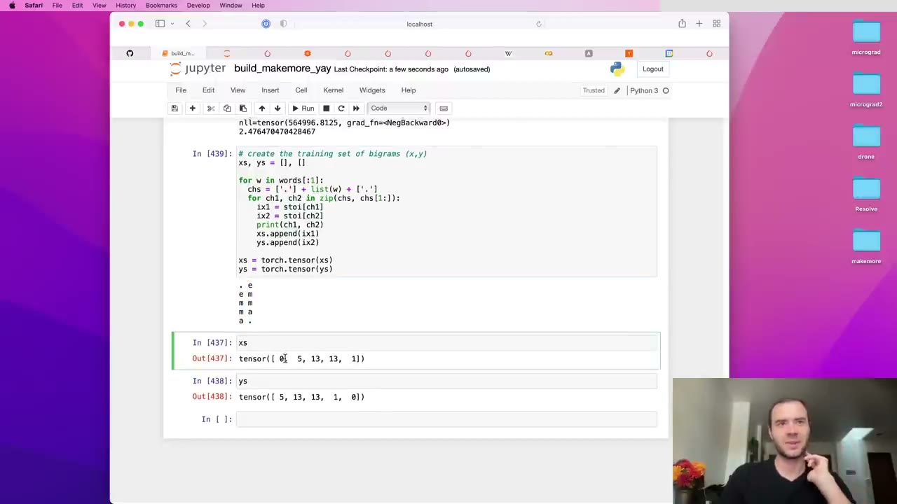
The training set reuses the bigram loop, but instead of counting it appends the first character’s index to xs and the second’s to ys (1:05:55), then converts both lists to tensors (1:06:27). To keep things readable it starts with only “emma”, which yields five examples: “.” to “e”, “e” to “m”, “m” to “m”, “m” to “a”, “a” to “.” (1:06:57). As integers, input 0 should give a high probability to 5, input 5 to 13, and so on (1:07:28).
A tangent on API traps (1:07:59): PyTorch has both torch.tensor and the class torch.Tensor, and the docs don’t make the difference clear (1:08:29). From a forum thread he finds that lowercase infers the dtype while capital always returns float32. Here lowercase gives integers, which is what indices should be, so he recommends lowercase (1:09:00), and uses the episode to encourage reading docs and threads with care.
1:10:02 – 1:13:39 One-hot encoding the inputs
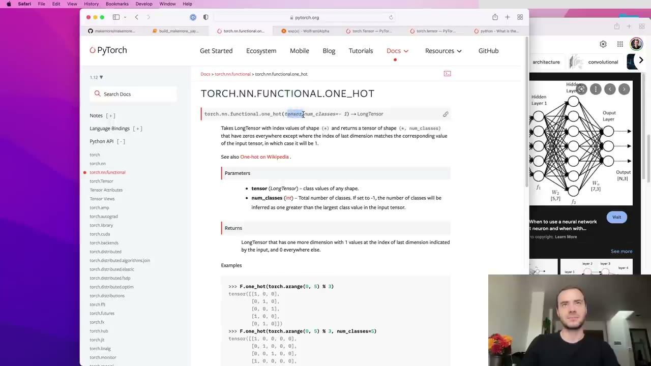
An integer index can’t sensibly be multiplied by weights (1:10:02), so the standard trick is one-hot encoding: a vector of zeros with a single one at the index (1:10:34). PyTorch provides it as F.one_hot in torch.nn.functional (1:11:04). Karpathy passes num_classes=27 explicitly, because otherwise it might guess a smaller size from the largest index present (1:11:36). The encoded “emma” examples, xenc, form a 5 by 27 matrix; plotted, each row lights up a single cell (1:12:07).
One more trap: xenc comes back as 64-bit integers (1:12:38), and one_hot takes no dtype argument, so he casts it with .float() before it goes into the network (1:13:09).
1:13:39 – 1:18:53 One linear layer as a matrix multiply
From micrograd, a neuron computes w·x + b (1:13:39). Karpathy starts with weights for one neuron from torch.randn, normally distributed values mostly near zero (1:14:12), shaped 27 by 1 (1:14:42). xenc @ W is a matrix multiply giving a 5 by 1 result (1:15:12): that one neuron evaluated on all five inputs in parallel (1:15:43).
Make W 27 by 27 and you have 27 neurons (1:16:14), with a 5 by 27 output (1:16:46). Entry [3, 13] is the 13th neuron’s response to the third input, the dot product of that input row with column 13 of W (1:17:16), which he confirms by computing it by hand (1:18:21). There is no bias, no tanh and no second layer: the whole network is one linear layer (1:18:53).
1:18:53 – 1:26:11 Logits, exponentiation and probabilities
The 27 outputs per example need a meaning (1:19:23). They are positive and negative, so they can’t be probabilities, which must be positive and sum to one (1:19:54), and they can’t be counts, which are positive integers (1:20:24). Karpathy’s choice: treat them as log counts. Exponentiating maps the whole real line to positive numbers, negatives to values below one and positives to values above (1:20:56), so the results can stand in for counts (1:21:57).
The standard name for these raw outputs is logits (1:23:03). logits.exp() plays the role of the old count matrix N, and dividing each row by its sum with keepdims=True, exactly as before, gives probabilities (1:23:34). Each of the five rows now sums to one (1:24:04). Every step, multiply, exponentiate, sum, divide, is differentiable, so the loss can be backpropagated to W (1:24:35). For the first example, feeding in “.” produces 27 probabilities for what comes next, and changing W changes them (1:25:39).
1:26:11 – 1:33:05 The forward pass, example by example
Karpathy gathers the pieces into one summary (1:26:11), now seeding the generator for W: one-hot inputs, a layer of 27 neurons that each see 27 inputs, logits, counts, probabilities (1:26:42). The last two steps, exponentiate and normalize, together are the softmax (1:27:14), a layer that turns any real-valued outputs into a probability distribution and can sit on top of any linear layer (1:27:45).
A printout walks through the five bigrams of “emma” (1:28:47). For “.” to “e”, input 0 goes in, label 5 picks out the probability of “e”, and the random network gives it only about 1% (1:29:52), a negative log likelihood near 4 (1:30:22). One pair happens to get 7%. The average over the five, 3.76, is the loss (1:31:25).
Changing the seed gives a different W and a loss of 3.37, another seed does worse (1:31:58). Karpathy calls this guess-and-check “amateur hour” (1:32:31). The real method uses the fact that the loss is differentiable: compute its gradient with respect to W and step downhill.
1:33:05 – 1:42:34 Vectorized loss, backward pass and update
The training loop will look almost identical to the end of micrograd, which Karpathy pulls up for comparison (1:33:05). There, four inputs went through an MLP and the loss was mean squared error (1:34:06); then gradients were zeroed, loss.backward() filled them in, and every parameter was nudged against its gradient (1:35:10). Here the network is a linear layer plus softmax, and because this is classification rather than regression, the loss is negative log likelihood (1:35:41).
To pick out the probability of the correct label for every example at once, he indexes probs with two tensors: torch.arange(5) for the rows and ys for the columns (1:37:19). Take .log(), .mean(), and negate, and the result matches the 3.76 from the loop (1:37:51).
The backward pass (1:38:22): reset the gradient by setting W.grad = None, which PyTorch treats as zero and is more efficient (1:38:52). W must be created with requires_grad=True so PyTorch tracks it (1:39:25). Then loss.backward() walks the computation graph PyTorch recorded during the forward pass, just as micrograd did (1:39:57). W.grad has the same 27 by 27 shape, and each entry says how nudging that weight would change the loss; a positive value means increasing the weight raises the loss (1:40:31).
The update copies micrograd almost exactly: W.data += -0.1 * W.grad (1:41:34). Forward again and the loss drops from 3.76 to 3.74, then 3.72 (1:42:04). That is gradient descent.
1:42:34 – 1:47:51 Training on all 228,000 bigrams
Karpathy rearranges everything into two cells, dataset plus initialization and a gradient-descent loop (1:42:34), with a counter showing five examples (1:43:06). Switching from “emma” to all words gives about 228,000 bigrams, and none of the code needs to change (1:43:38). The loss falls slowly, so he raises the learning rate; even 50 works on this simple problem (1:44:13).
What should the loss approach? The counting model scored about 2.45, or about 2.47 smoothed (1:44:44), and the network lands around 2.46 to 2.45 (1:45:15). That makes sense: it gets the same information, the previous character, so it can’t do better. Counting just happens to solve the bigram case directly (1:45:46).
The gain is flexibility (1:46:17). Future networks will take several previous characters and get far more complex, but they will still output logits that pass through softmax and the same loss and update (1:46:48). The counting approach can’t follow: with ten characters of context, the table of combinations becomes far too big to store (1:47:19).
Our note: with 27 symbols and 10 characters of context, the table would need 27¹⁰ rows, roughly 2 × 10¹⁴.
1:47:51 – 1:54:36 W is the count table, and regularization is smoothing
Two observations tie the approaches together. First, multiplying a one-hot vector by W just plucks out one row of W (1:47:51). That is exactly the table lookup of the counting model, where the first character selected a row (1:48:55). Since W holds log counts, W.exp() corresponds to the count array (1:49:26): one was filled in by counting, the other reached piece by piece by following the loss (1:49:57).
Our note: strictly, the match is only up to a scale factor per row. Softmax ignores adding the same constant to a whole row of logits, so gradient descent pins down each row’s shape but not its overall size.
Second, smoothing has a counterpart (1:50:28). Adding a huge fake count to every cell makes each row nearly uniform (1:50:59). In the network, if every weight is zero, the logits are zero, the counts are one, and the probabilities are exactly uniform (1:51:30). So pulling W toward zero is a form of smoothing. That leads to regularization (1:52:00): add a term such as 0.01 * (W**2).mean() to the loss, which is zero only when all weights are zero (1:52:31). He uses the mean rather than the sum to keep it manageable, and the 0.01 sets the strength (1:53:02).
Karpathy describes the term as a spring or gravity pulling the weights to zero, opposed by the data pulling the probabilities toward the real statistics (1:53:34). Turning up its strength is the analogue of adding more fake counts; make it strong enough and every prediction goes uniform (1:54:04).
Our note: in this passage Karpathy says “label smoothing”, but what he describes is the add-count smoothing from earlier. In current usage, label smoothing usually means softening the target labels, a different technique. The squared-weight penalty itself is L2 regularization, closely related to weight decay.
1:54:36 – 1:57:42 Sampling from the network, and what comes next
The sampling loop from earlier needs one change (1:54:36): instead of reading row ix of P, one-hot encode ix, multiply by W, exponentiate and normalize (1:55:07). With the same seed, the output names are the same as the counting model’s (1:55:37), because the two are essentially the same model reached by very different routes (1:56:08).
The wrap-up restates the arc (1:56:38): a bigram model trained by counting and by gradient descent, sampled and evaluated with negative log likelihood. From here the networks will take more characters and grow in complexity, but logits, normalization, loss and the gradient-based framework stay identical, all the way to transformers (1:57:10).
Our note: in Lecture 3 the hand-written softmax and negative log likelihood are replaced by PyTorch’s F.cross_entropy, which computes the same thing more efficiently and stably.
Code you’ll write
These are short excerpts in the style of the lecture notebook. The full code is lectures/makemore/makemore_part1_bigrams.ipynb in karpathy/nn-zero-to-hero, and the finished, more general model is in karpathy/makemore, both MIT-licensed.
1. Count every bigram into a 27 by 27 table (22:21). One “.” token marks both start and end, at index 0.
words = open('names.txt', 'r').read().splitlines()
N = torch.zeros((27, 27), dtype=torch.int32)
chars = sorted(list(set(''.join(words))))
stoi = {s: i+1 for i, s in enumerate(chars)}
stoi['.'] = 0
itos = {i: s for s, i in stoi.items()}

for w in words:
    chs = ['.'] + list(w) + ['.']
    for ch1, ch2 in zip(chs, chs[1:]):
        N[stoi[ch1], stoi[ch2]] += 1
2. Normalize rows and sample names (31:46). The +1 is the smoothing added at 1:01:49, and keepdims=True is what makes the division run along rows.
P = (N + 1).float()
P /= P.sum(1, keepdims=True)

g = torch.Generator().manual_seed(2147483647)
for i in range(5):
    out, ix = [], 0
    while True:
        ix = torch.multinomial(P[ix], num_samples=1, replacement=True, generator=g).item()
        out.append(itos[ix])
        if ix == 0:
            break
    print(''.join(out))
3. Average negative log likelihood over the training set (57:12).
log_likelihood = 0.0
n = 0
for w in words:
    chs = ['.'] + list(w) + ['.']
    for ch1, ch2 in zip(chs, chs[1:]):
        prob = P[stoi[ch1], stoi[ch2]]
        log_likelihood += torch.log(prob)
        n += 1
nll = -log_likelihood
print(f'{nll/n}')  # 2.476 with the +1 smoothing; 2.454 without
4. Build the (input, label) training set and initialize W (1:05:55).
xs, ys = [], []
for w in words:
    chs = ['.'] + list(w) + ['.']
    for ch1, ch2 in zip(chs, chs[1:]):
        xs.append(stoi[ch1])
        ys.append(stoi[ch2])
xs = torch.tensor(xs)
ys = torch.tensor(ys)
num = xs.nelement()

g = torch.Generator().manual_seed(2147483647)
W = torch.randn((27, 27), generator=g, requires_grad=True)
5. Train the one-layer network by gradient descent (1:42:34). The regularization term is added at 1:53:02.
import torch.nn.functional as F

for k in range(100):
    xenc = F.one_hot(xs, num_classes=27).float()  # one-hot inputs
    logits = xenc @ W                               # log-counts
    counts = logits.exp()                           # equivalent to N
    probs = counts / counts.sum(1, keepdims=True)   # softmax
    loss = -probs[torch.arange(num), ys].log().mean() + 0.01*(W**2).mean()

    W.grad = None
    loss.backward()
    W.data += -50 * W.grad
6. Sample from the trained network (1:55:07). Only the line that produces p differs from snippet 2.
g = torch.Generator().manual_seed(2147483647)
for i in range(5):
    out, ix = [], 0
    while True:
        xenc = F.one_hot(torch.tensor([ix]), num_classes=27).float()
        counts = (xenc @ W).exp()
        p = counts / counts.sum(1, keepdims=True)
        ix = torch.multinomial(p, num_samples=1, replacement=True, generator=g).item()
        out.append(itos[ix])
        if ix == 0:
            break
    print(''.join(out))
Our note: both spellings appear on screen and in the notebook. The shape checks around 40:15 and the first normalization at 44:00 use keepdim=True, PyTorch’s documented name; from 49:53 on, the normalization lines use keepdims=True. PyTorch accepts both.
Skip list
- 6:44 – 8:17 How
zippairs consecutive characters. Skip if you write Python every day. - 13:32 – 15:08 Creating and indexing a small tensor. Basic PyTorch.
- 18:41 – 20:49 The plotting code for the count table, and
.item(). Look at the picture, skip the Matplotlib. - 26:36 – 30:12
torch.multinomialon a toy three-element distribution. The real use follows right after. - 1:07:59 – 1:10:02
torch.tensorversustorch.Tensor. The takeaway is one line: use lowercase. - 1:31:58 – 1:32:31 Re-rolling the random seed to see different losses, which only sets up why guess-and-check is a bad idea.
- 1:56:38 – end Recap of the lecture.
Don’t skip 36:20 – 50:17. The broadcasting section is the part most people need on a rewatch.
Glossary
- makemore — Karpathy’s repository for character-level models that generate more examples like those in a training file; this lecture builds its simplest version.
- Character-level language model — a model that treats text as a sequence of characters and predicts the next character from those before it.
- Bigram — a pair of consecutive tokens; a bigram model predicts the next character from only the current one.
- Special token (‘.’) — an extra symbol padding each name at both ends, so the model learns which letters start and end names.
- stoi / itos — the lookup dictionaries from characters to integer indices and back.
- Broadcasting — PyTorch’s rule for combining tensors of different shapes by aligning dimensions from the right and stretching size-1 or missing ones.
- keepdim — an argument to reductions like
sumthat keeps the reduced dimension as size 1 instead of removing it; it decides which way a later broadcast runs. - torch.multinomial — samples integer indices according to a vector of probabilities.
- Likelihood — the product of the probabilities a model assigns to the observed data; higher means a better fit.
- Negative log likelihood (NLL) — minus the sum of log probabilities of the data; averaged over examples it is the loss used here, with 0 as the best value.
- Model smoothing — adding fake counts to every cell of a count table so no event gets zero probability.
- One-hot encoding — representing an index as a vector of zeros with a one at that position, so it can be fed into a network.
- Logits — a layer’s raw, unnormalized outputs, read here as log counts.
- Softmax — exponentiating logits and normalizing them to sum to one, turning any real-valued outputs into a probability distribution.
- Gradient descent — repeatedly computing the loss gradient with respect to the parameters and stepping the parameters against it.
- Regularization — an extra loss term that penalizes large weights; here it pushes predictions toward uniform, the network version of smoothing.
FAQ
What is a bigram language model in Karpathy's makemore lecture?
A model that predicts the next character from the single character before it and nothing else. Karpathy pads every name with a '.' token at the start and end, counts how often each pair of characters appears in 32,033 names, and turns each row of that 27 by 27 count table into a probability distribution. Sampling then walks the table one character at a time until it draws the '.' again.
Why does keepdim matter when normalizing the counts matrix?
P.sum(1, keepdims=True) returns a 27 by 1 column of row totals, which broadcasts across each row, so every row is divided by its own total. Without keepdims the result is a plain vector of 27, which broadcasting treats as a 1 by 27 row. The division still runs without an error, but it divides each column by the wrong totals, so the rows no longer sum to one. Karpathy uses this to show how silently broadcasting bugs can slip through.
What loss does the bigram model reach, and is that good?
Karpathy measures the average negative log likelihood over every bigram in the training set and gets about 2.45 for the counted table, or about 2.47 once add-one smoothing is applied. The neural network version converges to the same neighborhood. Our note: a model that guessed uniformly over 27 characters would score ln 27, about 3.30, so the bigram model has learned something, but its samples are still poor.
Why does Karpathy train the same bigram model twice?
Counting and normalizing gives the best bigram table directly, but it does not scale: with more characters of context the table explodes. Training a 27 by 27 weight matrix with softmax, negative log likelihood and gradient descent lands on essentially the same model and the same samples, and that machinery carries over unchanged to MLPs, RNNs and transformers, where only the forward pass gets more complex.
What is the difference between torch.tensor and torch.Tensor?
In the lecture, Karpathy finds that lowercase torch.tensor infers the data type from what you pass in, so a list of integers becomes an integer tensor, while the capital torch.Tensor class always gives float32. Since the training inputs and labels are character indices, he recommends sticking with lowercase torch.tensor.
Studying another course? Paste its YouTube or Bilibili link on the home page to request a handout — or make your own with the desktop app (coming soon).