Karpathy's Zero to Hero, Lecture 6: Building a WaveNet — notes, code and timestamps

Updated 2026-10-07 · Video: Andrej Karpathy, published 2022-11-21 · 56 min

46 key slides

Watch the video (56 min)

Lecture 6 of Andrej Karpathy’s Neural Networks: Zero to Hero series is the last makemore video, and it is less about a new idea than about growing an old one. Karpathy starts from the character-level MLP he left at the end of makemore Part 3 (Part 4, covered in Lecture 5, was the manual-backprop detour) and makes two changes: a longer context of eight characters, and a deeper network that fuses those characters a pair at a time instead of all at once. Along the way the notebook gets “PyTorch-ified” with Embedding, Flatten and Sequential modules, a quiet BatchNorm bug turns up when tensors go 3D, and validation loss falls from 2.10 to 1.993. The lecture ends with a preview of how the same model becomes a convolutional network, before the series turns to Transformers in Lecture 7.

Key takeaways

Squashing the whole context into one layer is the bottleneck (17:46). Making the single hidden layer bigger doesn’t fix the fact that all characters are mixed in one step.
A longer context alone buys a lot (20:54). Going from three to eight characters with the same flat MLP drops validation loss from 2.10 to about 2.02.
PyTorch’s matrix multiply treats every leading dimension as a batch (25:08). That is what lets one Linear layer process all character pairs in parallel.
A single view can do the regrouping (30:21). Reshaping (4, 8, 10) to (4, 4, 20) gives exactly the same result as concatenating even and odd positions by hand.
Same parameters, same loss: the tree isn’t automatically better (38:12). At about 22,000 parameters the hierarchical model scores 2.029 against 2.027 for the flat one.
Broadcasting can hide a real bug (40:47). BatchNorm ran without errors on 3D input but kept separate statistics for each position; reducing over two dimensions fixed it.
Convolutions are an efficiency trick, not a different model (47:33). They slide the same tree across a sequence and reuse shared intermediate values.

Chapter notes

0:02 – 1:35 From a three-character MLP to a WaveNet

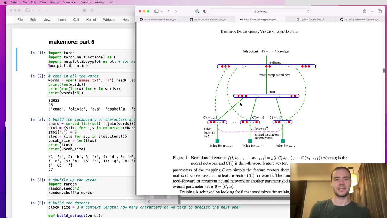
Karpathy is recording from a hotel room in Kyoto. The starting point is the model from the previous makemore lectures: three characters in, one hidden layer of tanh neurons, a guess at the fourth character. The plan for this video is to feed in more characters and, more importantly, stop fusing them all in the first layer. A deeper network that merges information progressively ends up looking much like WaveNet (1:03), the 2016 DeepMind paper. WaveNet predicts audio samples rather than characters, but the setup is the same: an autoregressive model that predicts the next item in a sequence, here with a tree-shaped hierarchy.

Bengio et al. paper, Figure 1: three character embeddings looked up in table C feed one tanh hidden layer and a softmax output, shown beside the makemore part 5 notebook — 0:17 — The starting point: the Bengio-style MLP from the earlier lectures, where all context characters are concatenated and mixed in a single tanh layer.

1:35 – 6:48 The starter code and why BatchNorm is a “weird” layer

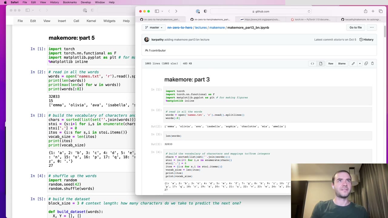
The starter notebook is lifted from Part 3 with few changes: the same names dataset, about 182,000 training examples of “three characters, predict the fourth”, and the hand-written layer classes (Linear, BatchNorm1d, Tanh) whose interfaces deliberately mimic torch.nn.

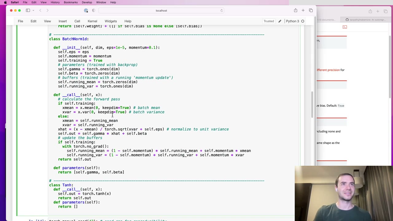
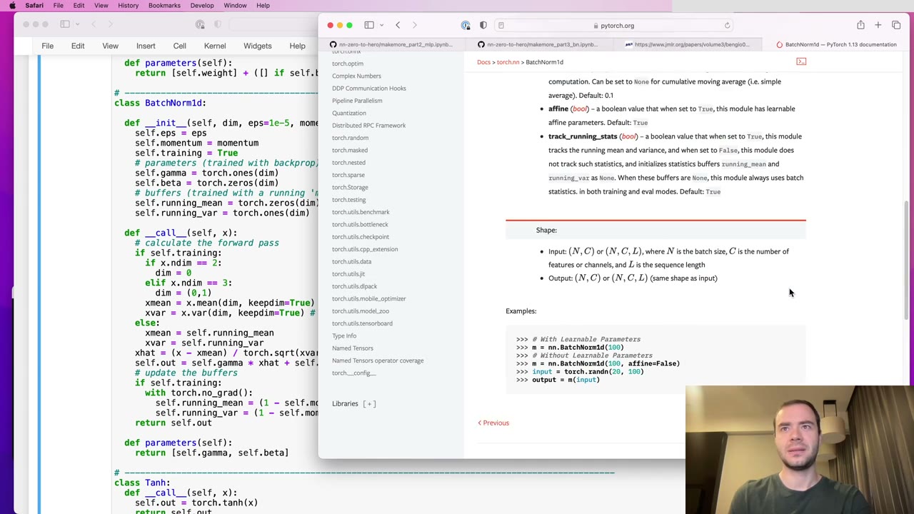
GitHub page for nn-zero-to-hero/lectures/makemore/makemore_part3_bn.ipynb showing the 'makemore: part 3' notebook, next to the new 'makemore: part 5' notebook — 1:42 — The Part 3 notebook on GitHub, which the starter code for this lecture is copied from.

Karpathy pauses on BatchNorm because it will bite twice in this video (3:42). It carries running mean and variance that are updated by an exponential moving average rather than by backprop; it has a training flag, because it behaves differently in training and evaluation; and it couples the examples in a batch, so the batch is no longer just an efficiency device. His summary of the lesson: state inside a layer is usually harmful. He also drops the per-layer generator objects in favour of seeding the torch RNG once globally (4:44).

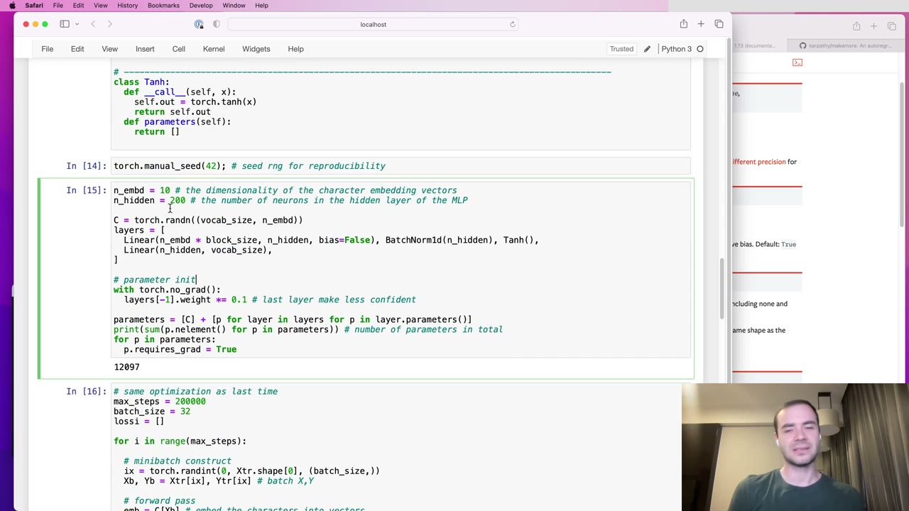
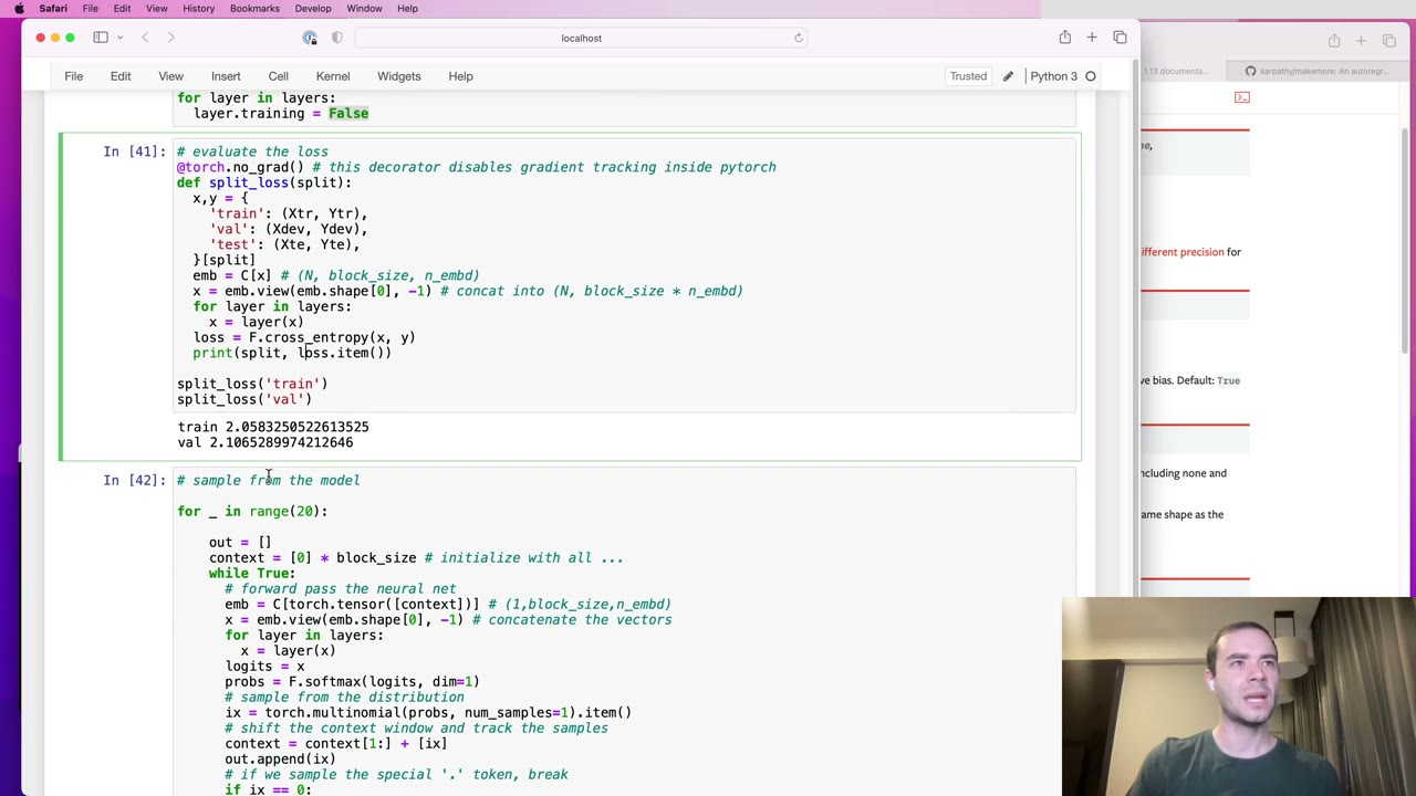
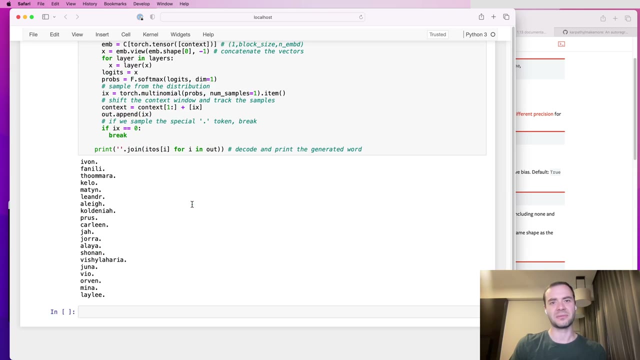
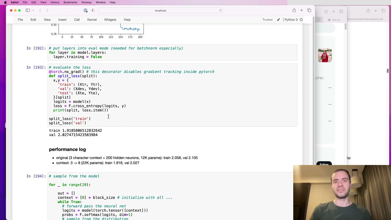
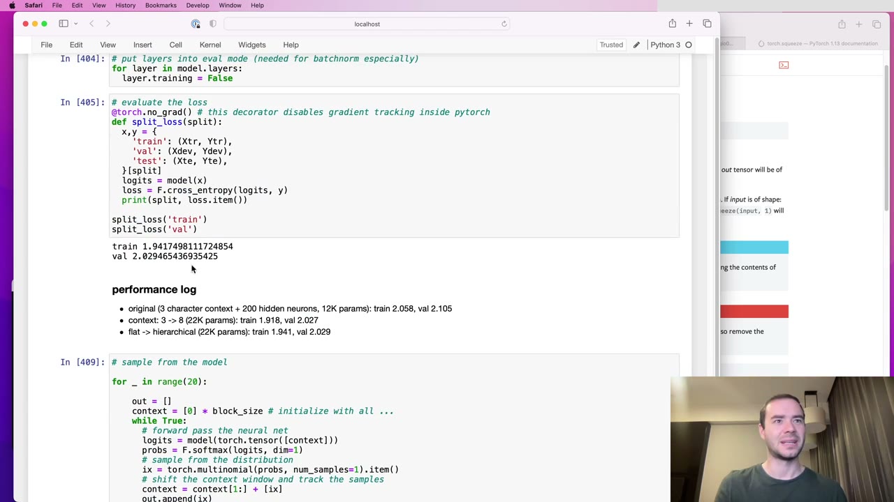
BatchNorm1d class in the notebook: __init__ with eps, momentum, a training flag, gamma, beta, running_mean and running_var; __call__ using x.mean(0) and x.var(0) in training mode, running statistics otherwise, and momentum updates of the buffers under torch.no_grad() — 3:40 — The Part 3 BatchNorm1d: a training flag, buffers updated outside backprop, and batch statistics taken over dimension 0 only, which is the detail that breaks later in the video.

The baseline (5:15) is an embedding table, Linear, BatchNorm, tanh and an output layer scaled down at initialization, about 12,000 parameters. It reaches a validation loss of 2.10 (6:17) and produces samples that sound plausible but not great.

Model cell: n_embd = 10, n_hidden = 200, C = torch.randn((vocab_size, n_embd)), layers = [Linear(n_embd * block_size, n_hidden, bias=False), BatchNorm1d(n_hidden), Tanh(), Linear(n_hidden, vocab_size)], last layer weight scaled by 0.1, printed parameter count 12097 — 5:18 — The baseline: an embedding table C kept outside a plain list of layers, 12,097 parameters in total.

split_loss cell output: train 2.0583250522613525, val 2.1065289974212646 — 6:20 — Baseline losses after training: train 2.058, validation 2.107.

Sampling cell output: twenty generated names such as ivon, fanili, thoommara, kelo, carleen, jorra, alaya, vishylaharia, orven, laylee — 6:30 — Samples from the baseline: name-like, but many are clearly off.

6:48 – 12:32 A readable loss curve, and the Embedding and Flatten modules

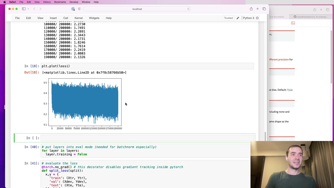
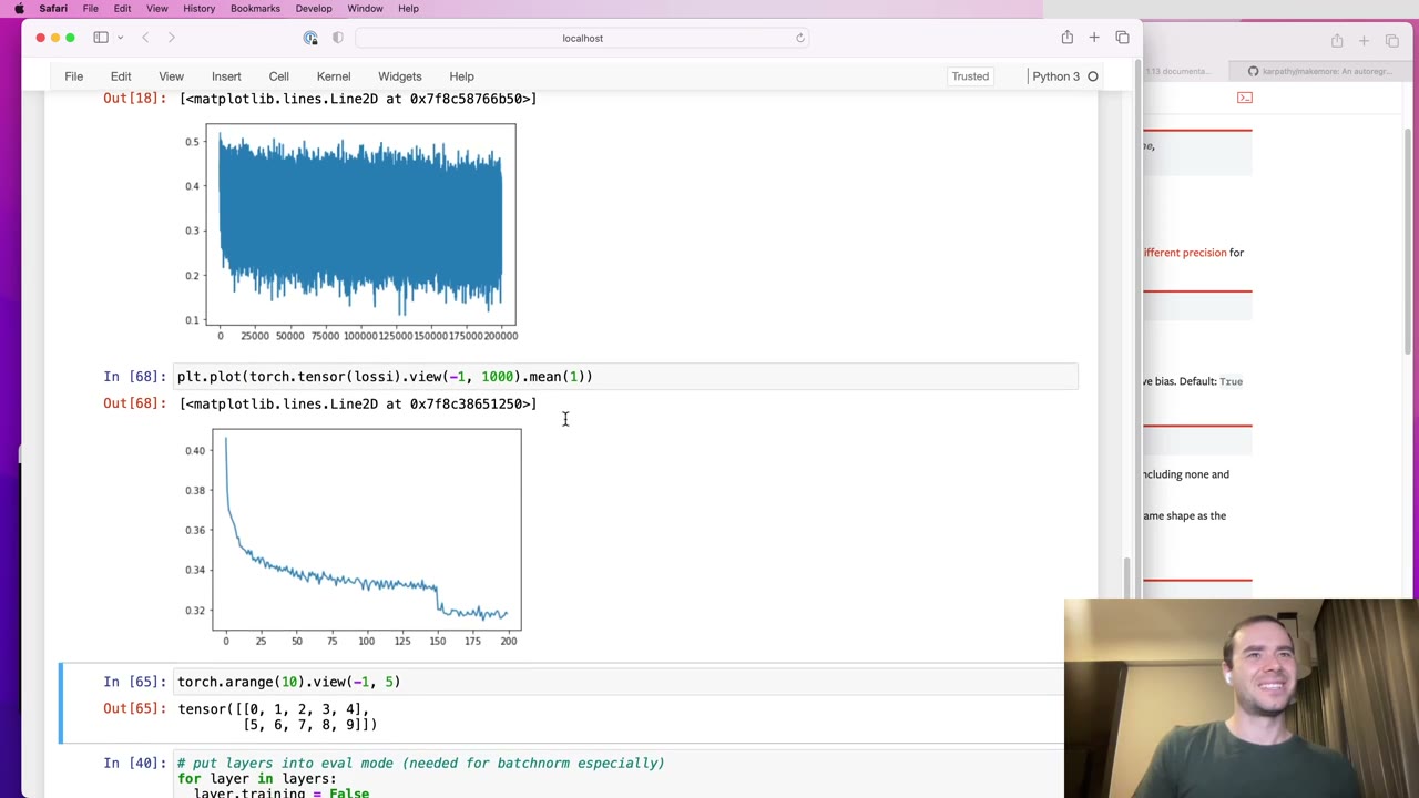
First a cosmetic fix. With batches of 32, the per-step loss jumps around so much that the plot is a thick smear. The trick (8:21) is to turn the list of 200,000 losses into a tensor, view it as 200 rows of 1,000 consecutive values, and average each row. The smoothed curve shows something the smear hid: the learning-rate decay late in training visibly settles the loss into a lower minimum (8:51).

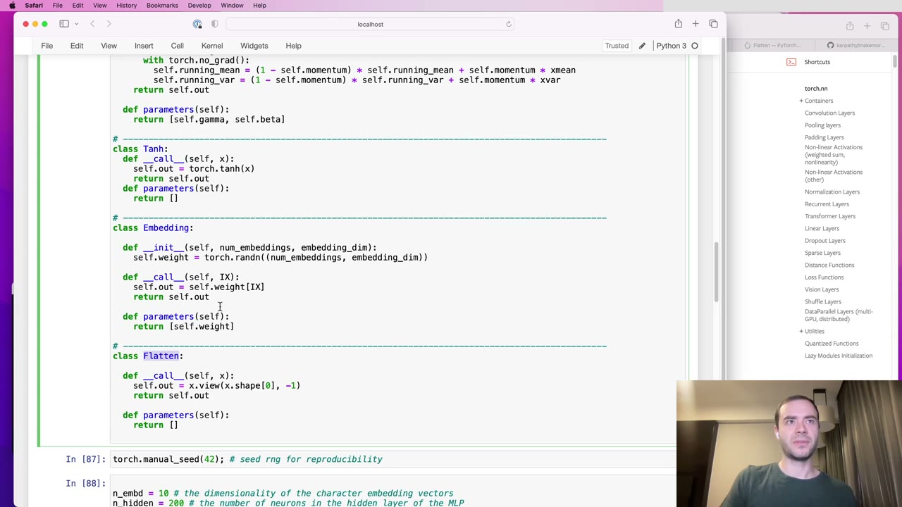
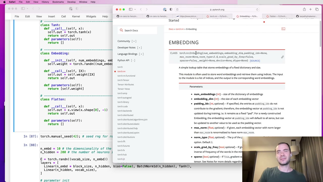
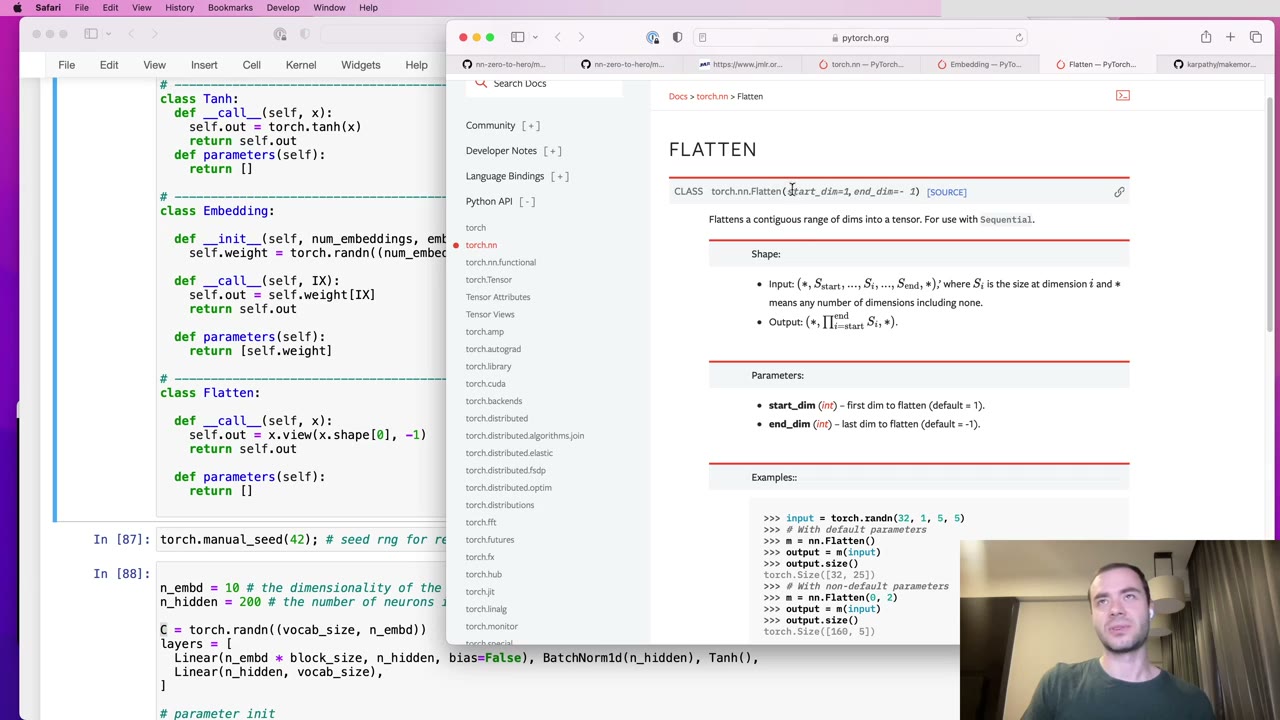
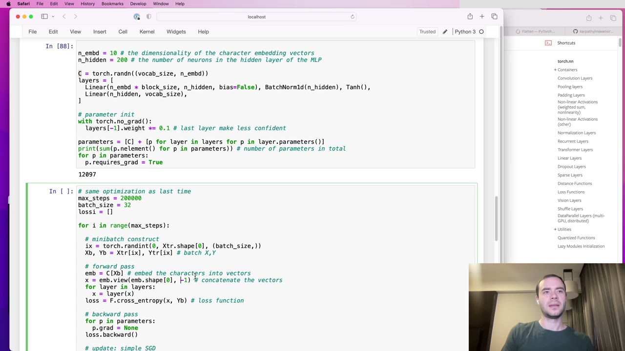
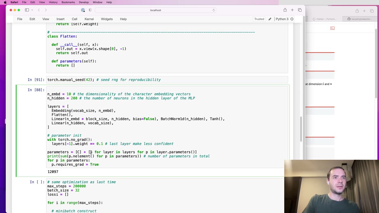
plt.plot(lossi) output: a dense blue band of per-step log losses over 200,000 steps, roughly 0.1 to 0.5 — 7:01 — The raw loss plot: with batches of 32 the per-step values form a thick band that hides the trend.

Cell plt.plot(torch.tensor(lossi).view(-1, 1000).mean(1)) and its plot: a smooth curve falling from about 0.40 to 0.33, with a sudden drop near x = 150, above a torch.arange(10).view(-1, 5) example — 8:55 — The smoothed curve: averaging 1,000-step blocks shows steady progress and the step down where the learning rate decays at 150,000.

Next, the forward pass still had two special cases sitting outside the layer list: indexing into the embedding table C, and the view that stretches the embeddings into one row (9:53). Karpathy wraps them as Embedding and Flatten modules (10:24), noting that both exist in PyTorch with many more keyword arguments. Now C becomes the embedding module’s weight, and the raw integer batch can go straight into the first layer.

New Embedding class (weight = torch.randn((num_embeddings, embedding_dim)), __call__ returns self.weight[IX]) and Flatten class (__call__ returns x.view(x.shape[0], -1)), each with a parameters() method — 10:42 — The two new modules: Embedding owns the lookup table as weight, and Flatten does the view.

PyTorch documentation page for torch.nn.Embedding, showing the signature with num_embeddings, embedding_dim, padding_idx, max_norm and other arguments — 11:05 — PyTorch's own Embedding, with many more keyword arguments than the minimal version written here.

PyTorch documentation page for torch.nn.Flatten(start_dim=1, end_dim=-1), with shape description and examples — 11:21 — PyTorch's Flatten, whose start_dim and end_dim arguments the hand-written version leaves out.

Training-loop cell with the forward pass emb = C[Xb] and x = emb.view(emb.shape[0], -1) written outside the for layer in layers loop — 10:17 — The two special cases in the forward pass: the lookup into C and the view that concatenates the embeddings, both outside the layer list.

Model cell where layers = [Embedding(vocab_size, n_embd), Flatten(), Linear(n_embd * block_size, n_hidden, bias=False), BatchNorm1d(n_hidden), Tanh(), Linear(n_hidden, vocab_size)], parameter count 12097 — 11:53 — The layer list now starts with Embedding and Flatten; the parameter count stays at 12,097.

12:32 – 17:15 A Sequential container, and a bug from forgotten state

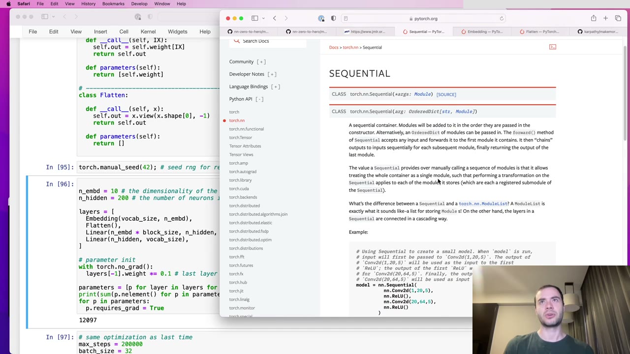
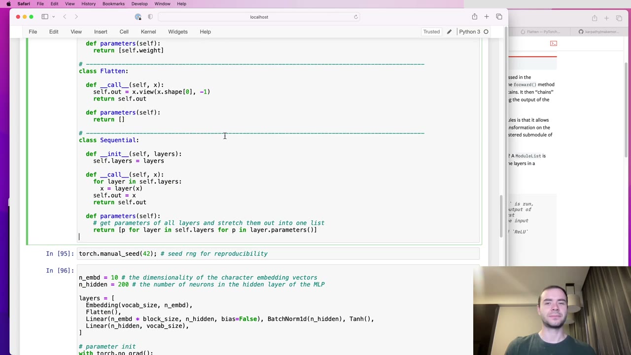
PyTorch organizes layers in containers, and the simplest is Sequential: hold a list of layers, pass the input through each in turn, and collect every child’s parameters (13:03). With a hand-written version, the whole network becomes one model object, the forward pass is logits = model(Xb), and evaluation and sampling shrink the same way.

PyTorch documentation page for torch.nn.Sequential, describing a sequential container that chains modules, with an example using nn.Conv2d and nn.ReLU — 13:18 — PyTorch's Sequential container, the model for the hand-written one.

New Sequential class: __init__ stores layers, __call__ passes x through each layer and stores self.out, parameters() returns [p for layer in self.layers for p in layer.parameters()] — 13:32 — The hand-written Sequential: run the layers in order and collect every child's parameters.

Model cell rewritten as model = Sequential([Embedding(vocab_size, n_embd), Flatten(), Linear(n_embd * block_size, n_hidden, bias=False), BatchNorm1d(n_hidden), Tanh(), Linear(n_hidden, vocab_size)]), parameters = model.parameters(), 12097 — 14:03 — The whole network is now one model object, and parameters come from model.parameters().

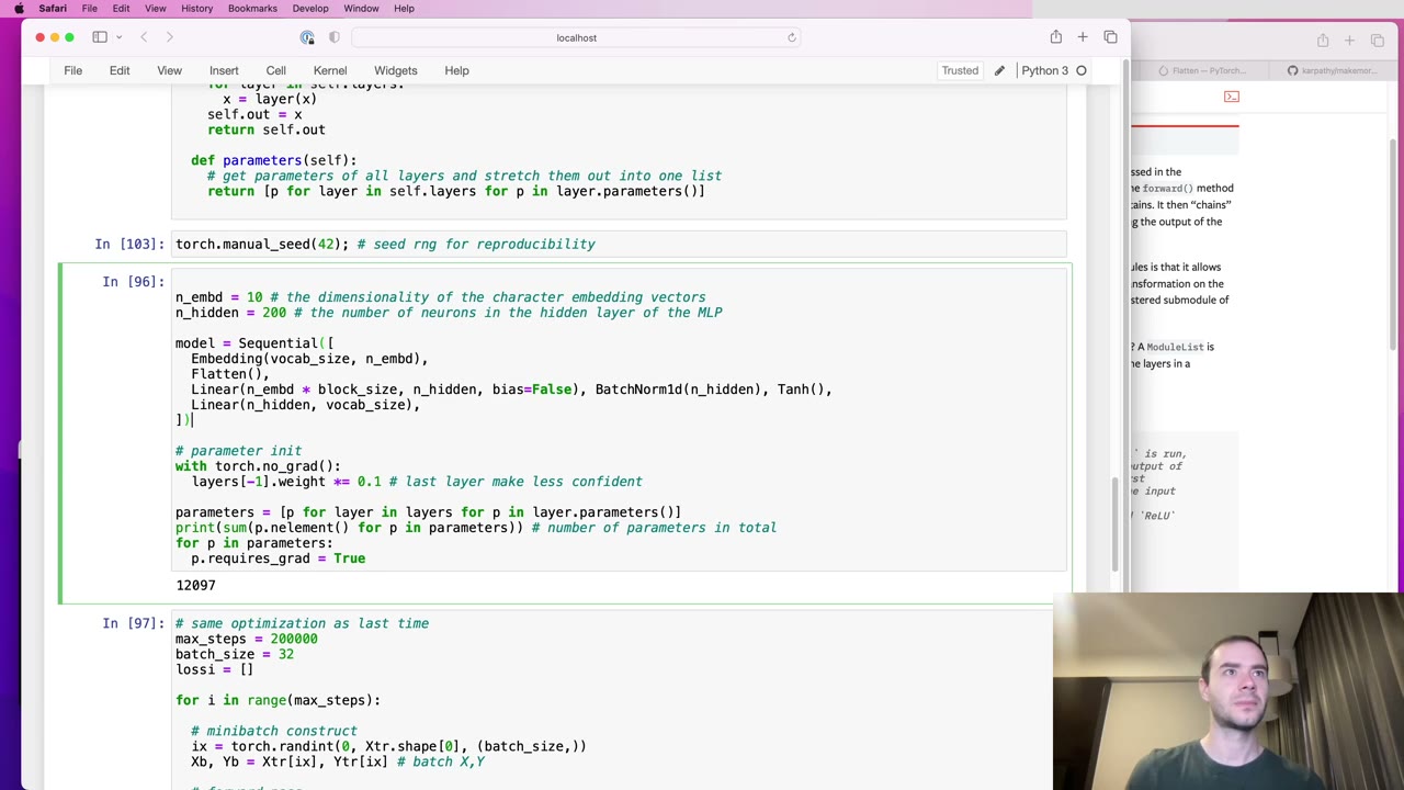
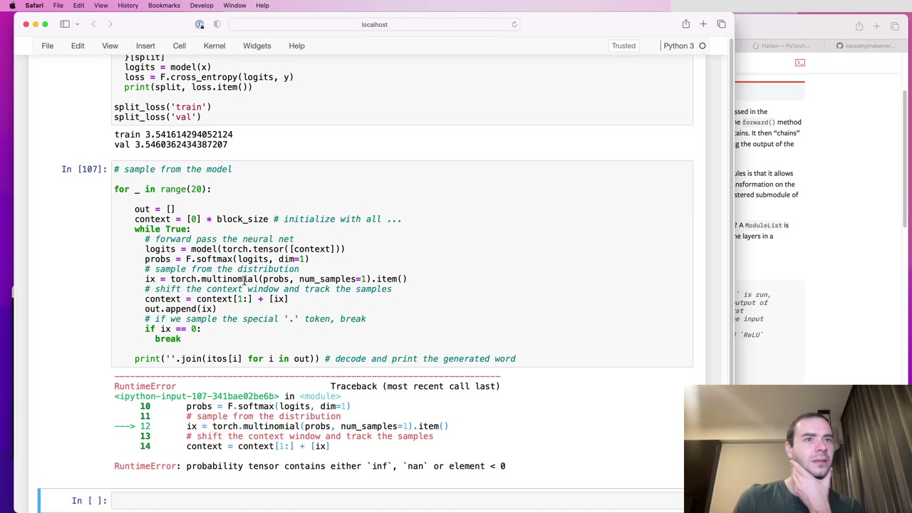
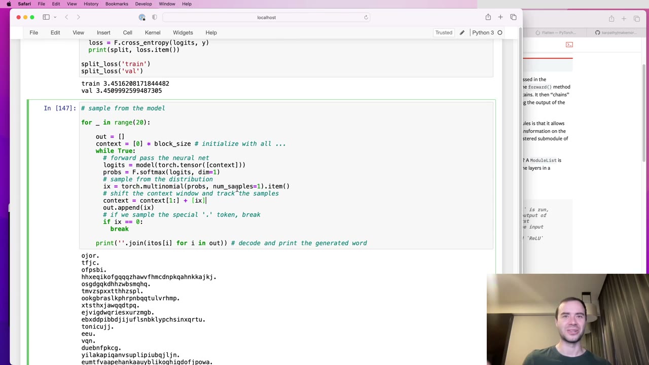
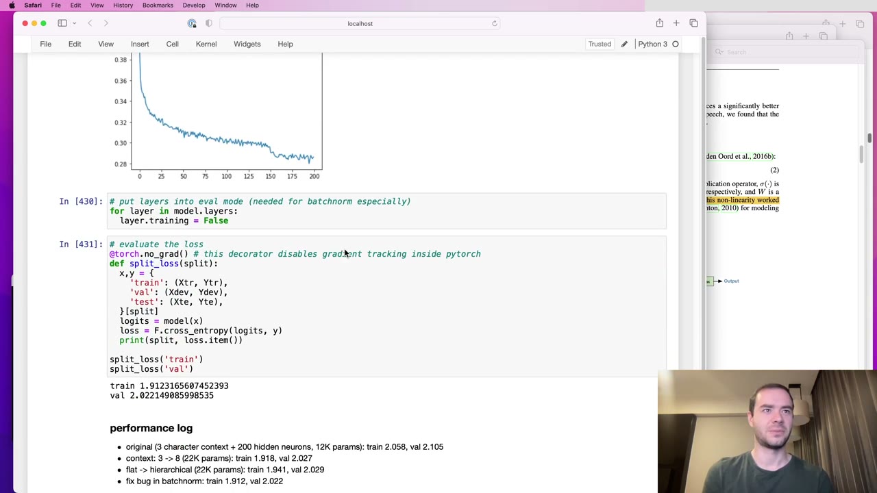
Then the sampling cell crashes with a RuntimeError (15:44). The cell that switches every layer to evaluation mode hadn’t been re-run after the refactor, so BatchNorm was still in training mode. Sampling feeds it a batch of one example, and the variance of a single number is NaN, which then poisons everything downstream (16:15). Karpathy points out the nastier version: when evaluating the loss you would get a number, just a wrong one, computed from batch statistics instead of the running ones. It’s the stateful-layer warning from the start, coming true.

Sampling cell output: RuntimeError traceback at torch.multinomial, 'probability tensor contains either inf, nan or element below 0'; the loss cell above shows train 3.54 and val 3.546 — 15:37 — The bug as it appeared: sampling crashes in torch.multinomial because BatchNorm, still in training mode, produced NaNs from a batch of one.

Sampling cell output after the fix: gibberish strings such as ojor, tfjc, hhxeqikofgqqqzhawvfhmcdnpkqahnkkajkj, eeu, vqn — 16:04 — Once the eval-mode cell is re-run, sampling works; the output is gibberish because the re-initialized model is untrained.

Our note: in real PyTorch, model.eval() and model.train() set this flag on every submodule at once, which is exactly the bookkeeping that went wrong here.

17:15 – 21:27 The WaveNet idea and a longer context

Training and validation losses are close (2.05 and 2.10), so the model isn’t overfitting and there’s room to scale up (17:15). The problem is how. Adding neurons or layers after the first one doesn’t change the fact that every character is crushed together immediately.

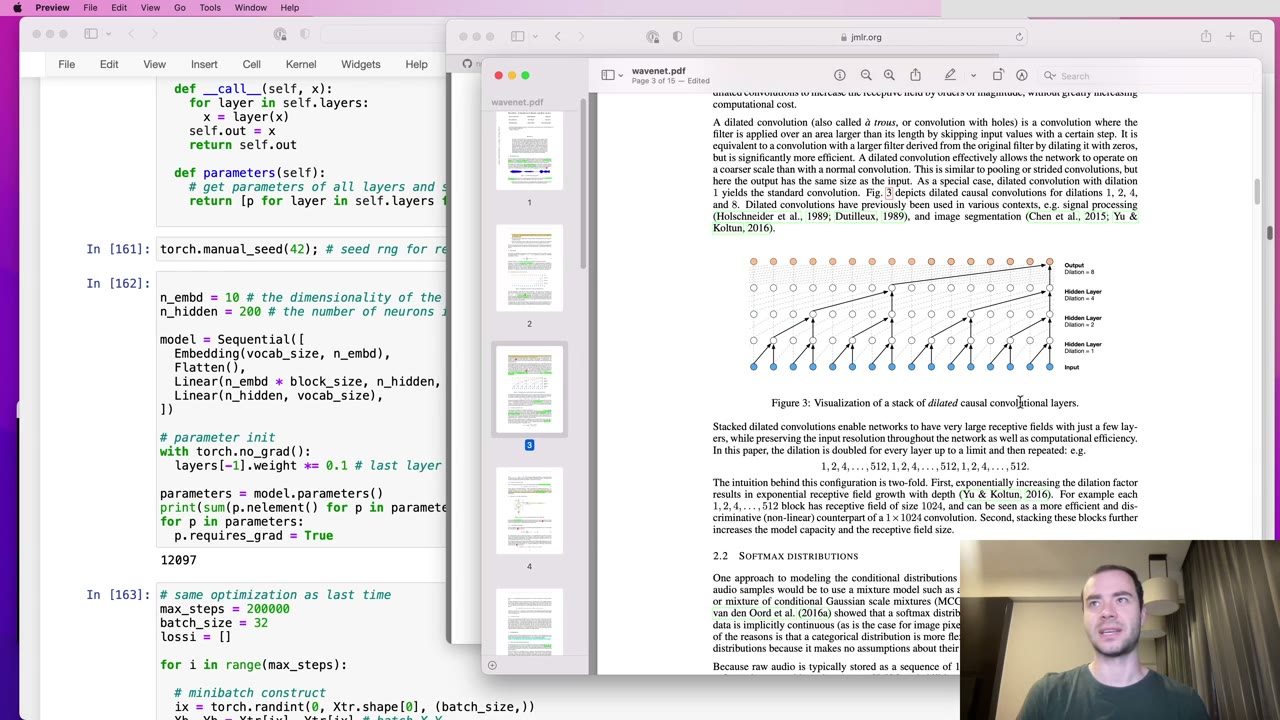
WaveNet’s figure shows the alternative (18:17): fuse two neighbouring characters into a bigram-like representation, then fuse pairs of those into four-character chunks, and so on up the tree. The paper’s labels say “dilated causal convolution”, which sounds intimidating, but Karpathy treats it as an implementation detail for speed (18:49) and keeps only the core idea of progressive fusion.

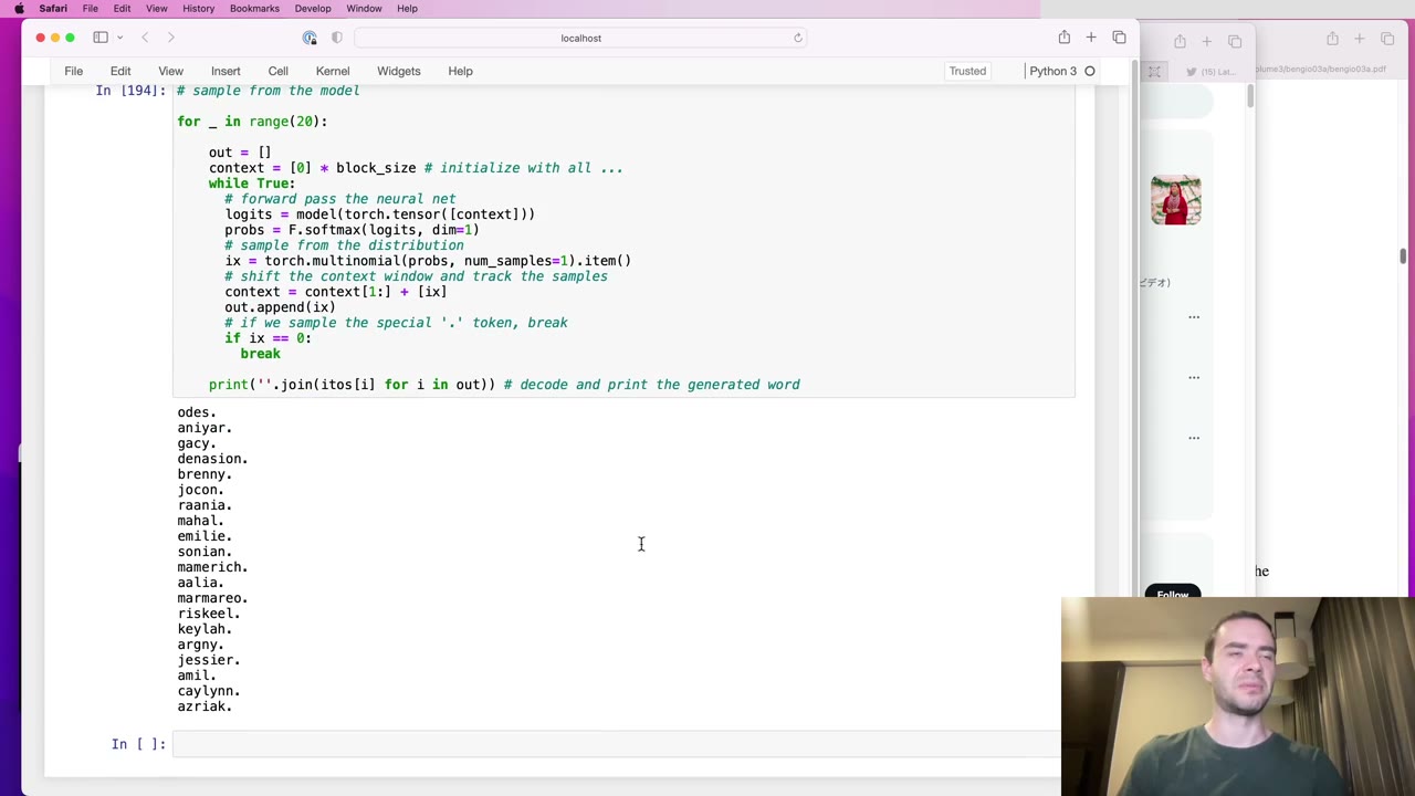
WaveNet paper PDF, Figure 3: visualization of a stack of dilated causal convolutional layers, with input, hidden layers at dilation 1, 2 and 4, and output at dilation 8 — 18:14 — WaveNet's Figure 3: inputs are fused in pairs, then pairs of pairs, up a tree to a single output.

Step one is changing block_size from 3 to 8 (19:20). The flat network still runs and its first Linear layer grows by about 10,000 parameters. Before going hierarchical, Karpathy trains this lazy version as a baseline and starts a performance log: 2.10 becomes about 2.02 (20:54), with visibly better names.

Dataset-printing cell output with block_size 8: rows like ........ → y, .......y → u up to ..yuheng → ., then ........ → d through .diondre → . — 19:43 — With block_size = 8 every example now carries eight characters of context, padded with dots at the start of a name.

split_loss output train 1.9185806512832642, val 2.0274715423583984, followed by a performance log: original (3 character context + 200 hidden neurons, 12K params): train 2.058, val 2.105; context: 3 → 8 (22K params): train 1.918, val 2.027 — 20:47 — The performance log starts: a context of 8 with the flat model gives validation 2.027, down from 2.105.

Sampling cell output from the block-size-8 model: names such as odes, aniyar, denasion, brenny, emilie, sonian, keylah, jessier, caylynn, azriak — 21:08 — Samples from the longer-context flat model.

21:27 – 28:14 Following the shapes through the network

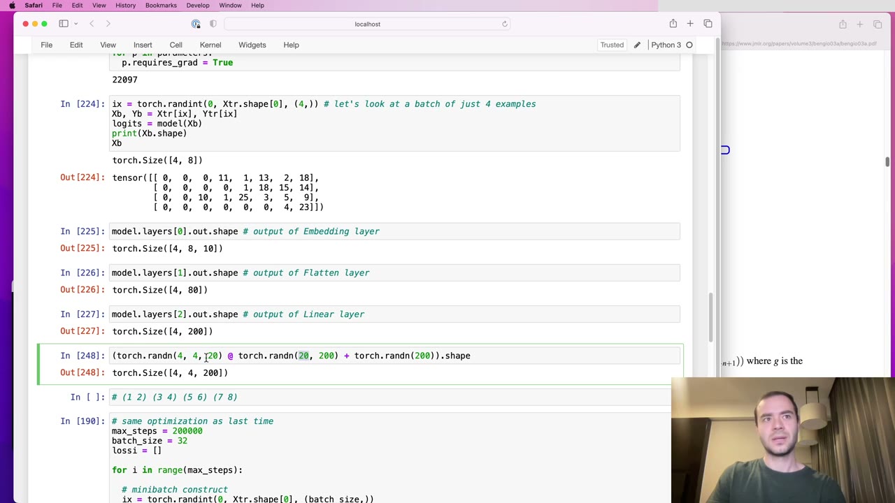
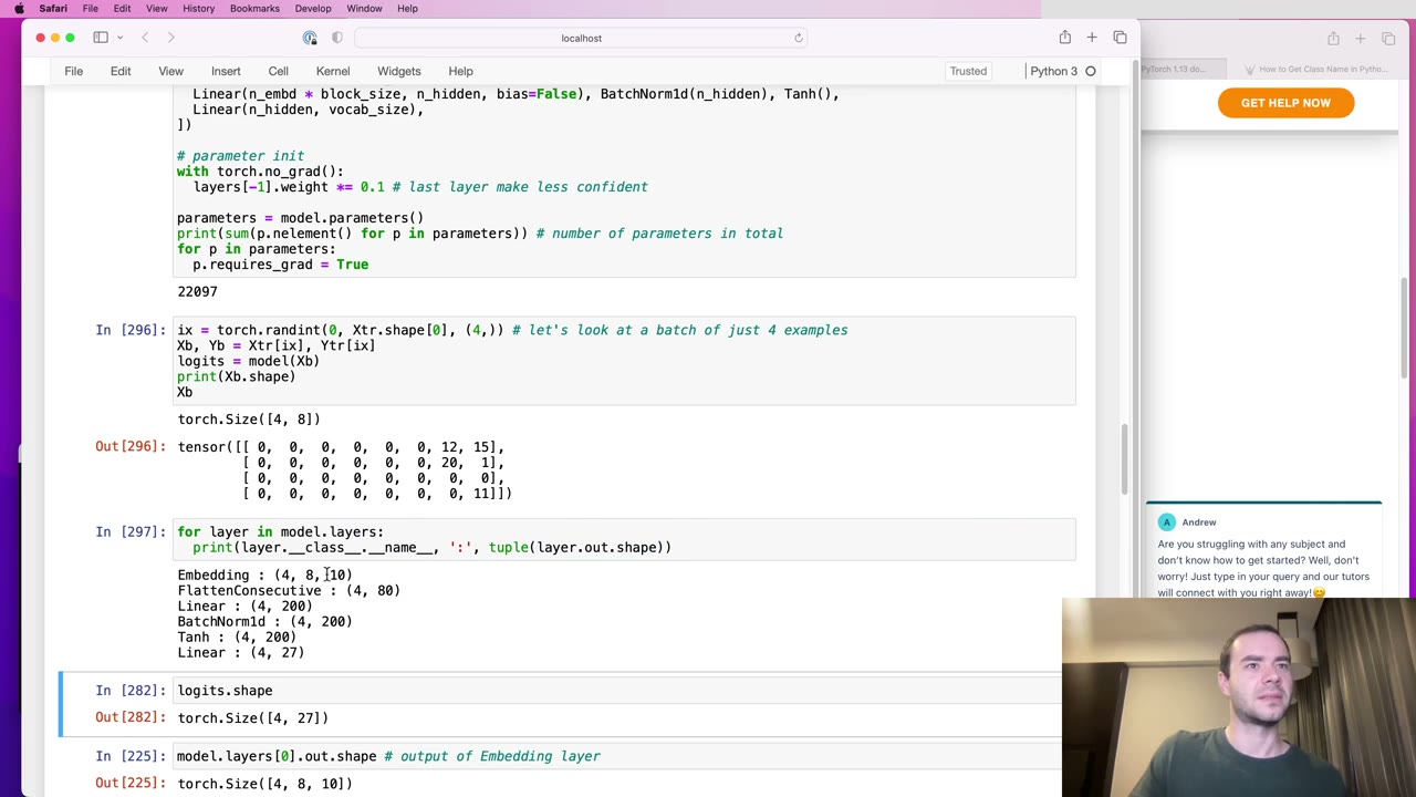
To design the change, Karpathy forwards a debug batch of four examples and prints shapes (21:58). The integer input is 4 × 8. The embedding layer turns it into 4 × 8 × 10, Flatten views that as 4 × 80, and Linear maps it to 4 × 200.

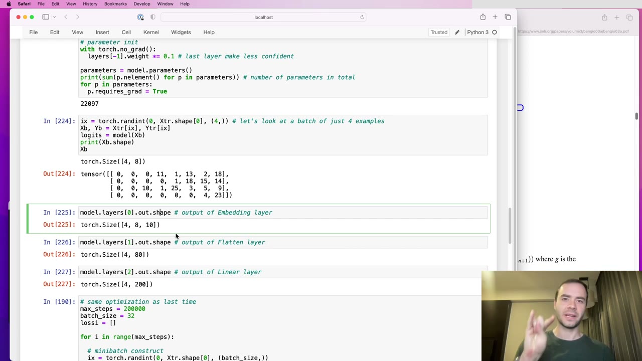
Debug cell: a batch of 4 examples, Xb shape torch.Size([4, 8]) with its integer rows, then model.layers[0].out.shape = [4, 8, 10] (Embedding), layers[1] = [4, 80] (Flatten), layers[2] = [4, 200] (Linear) — 22:44 — Shapes through the flat network for four examples: 4 × 8 integers, 4 × 8 × 10 embeddings, 4 × 80 after Flatten, 4 × 200 after Linear.

The surprise is inside Linear (24:36). The @ operator doesn’t require a 2D input. Give it 4 × 5 × 80 and an 80 × 200 weight, and out comes 4 × 5 × 200: the multiply acts on the last dimension and every dimension before it is treated as a batch (25:08).

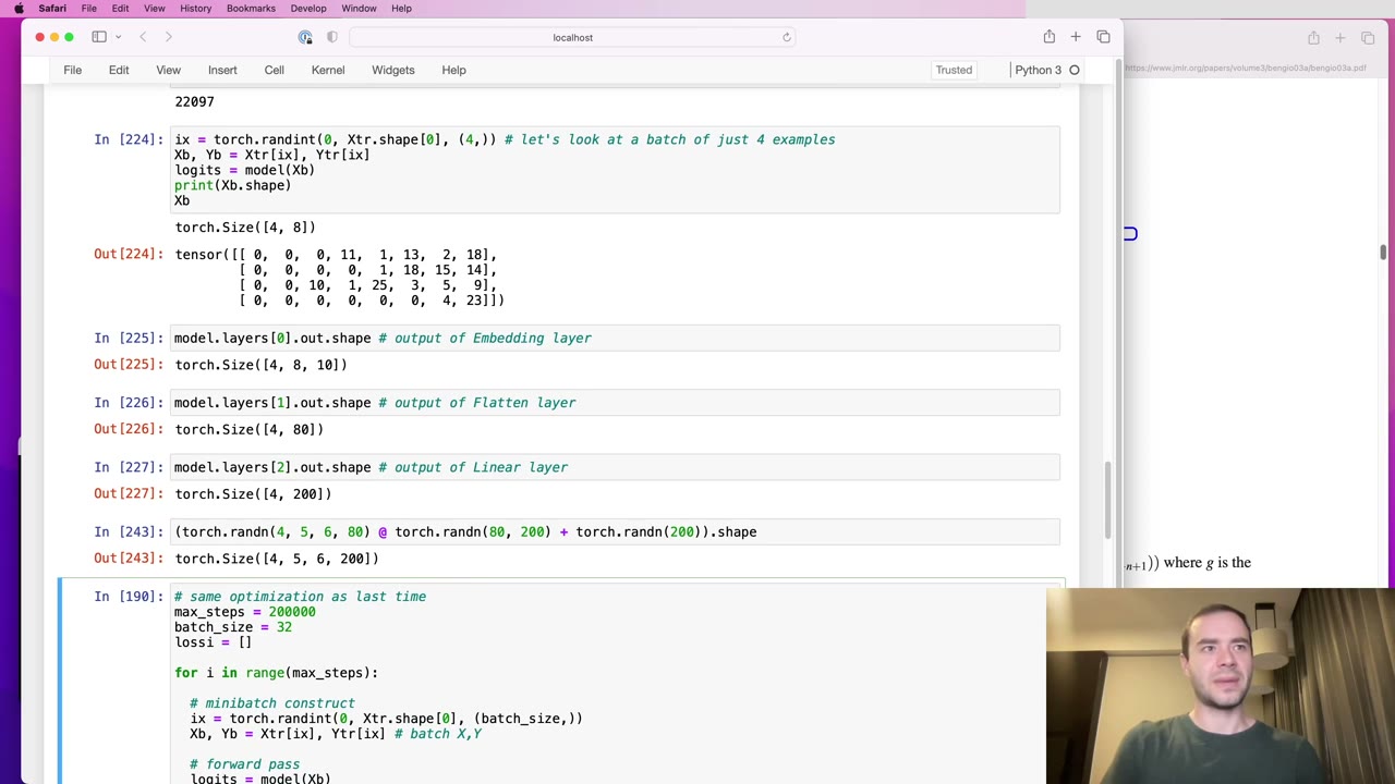
Cell (torch.randn(4, 5, 6, 80) @ torch.randn(80, 200) + torch.randn(200)).shape with output torch.Size([4, 5, 6, 200]) — 25:45 — Matrix multiply only touches the last dimension: even a 4 × 5 × 6 × 80 input comes out as 4 × 5 × 6 × 200.

That’s the lever for the tree. Rather than feed 80 numbers into the first layer, feed 20: one pair of 10-dimensional character vectors. The eight characters form four pairs, and those four groups become a second batch dimension, so the target input shape for the first Linear is 4 × 4 × 20 instead of 4 × 80 (27:13). Linear then needs 20 inputs, and Flatten has to stop flattening everything.

Cell (torch.randn(4, 4, 20) @ torch.randn(20, 200) + torch.randn(200)).shape with output torch.Size([4, 4, 200]), and a comment # (1 2) (3 4) (5 6) (7 8) below — 28:07 — The target shape: four pairs of 20 numbers per example, processed in parallel by a Linear layer with 20 inputs.

28:14 – 35:06 Writing FlattenConsecutive

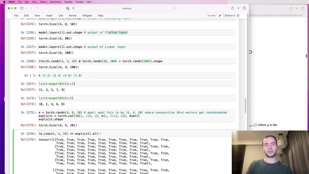
Karpathy first builds the 4 × 4 × 20 tensor the explicit way (29:18): take the even positions with a step-2 slice, the odd positions likewise, and concatenate along the last dimension. Then he shows that simply viewing the 4 × 8 × 10 tensor as 4 × 4 × 20 gives an identical result, element for element (30:21). Because consecutive vectors already sit next to each other in memory, a reshape is enough.

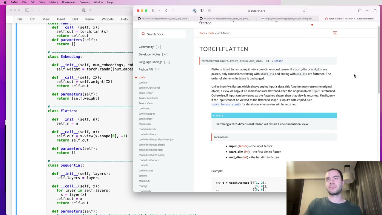
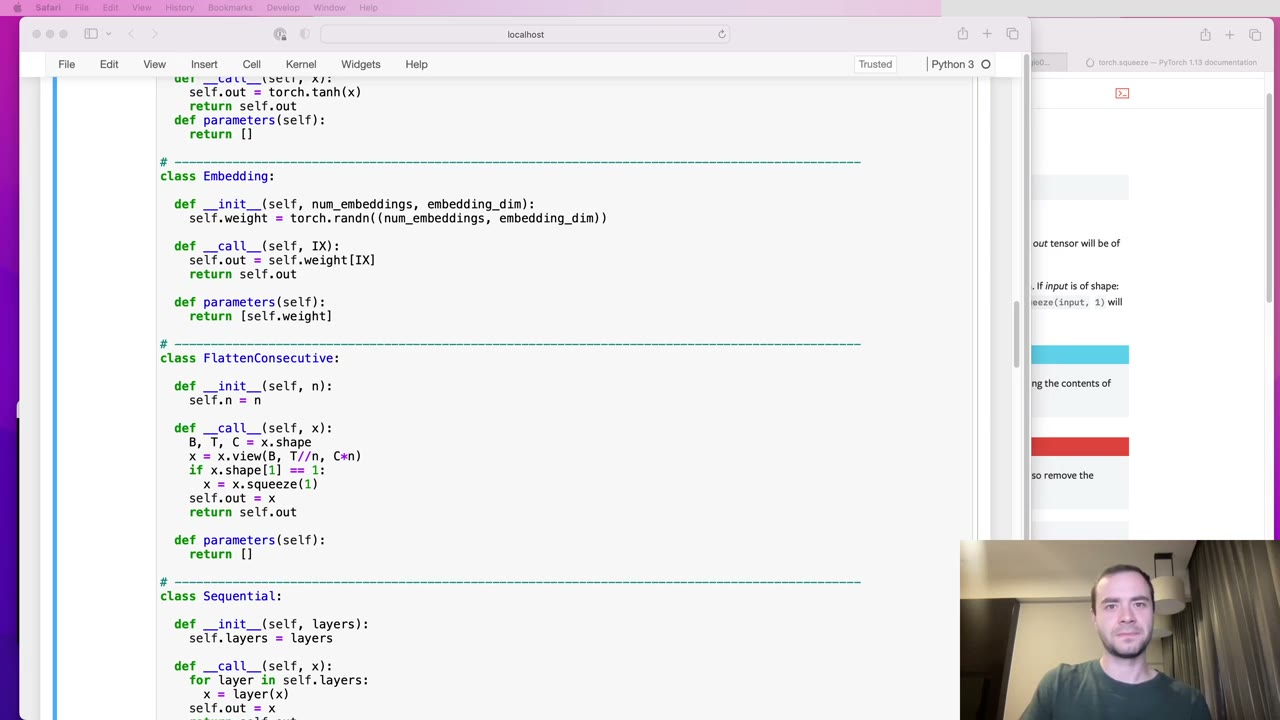
Cells list(range(10))[1::2] and [::2], then e = torch.randn(4, 8, 10) with explicit = torch.cat([e[:, ::2, :], e[:, 1::2, :]], dim=2) giving torch.Size([4, 4, 20]), and (e.view(4, 4, 20) == explicit).all() returning tensor(True) — 30:50 — The explicit even/odd concatenation and the one-line view produce identical 4 × 4 × 20 tensors.

The new layer (31:24) takes n, the number of consecutive elements to merge. Since its behaviour now differs from PyTorch’s Flatten, he renames it FlattenConsecutive (31:54). Two design choices are worth copying. He writes the middle dimension as T // n rather than -1, because an explicit shape raises an error when your assumptions are wrong (32:56). And if only one group is left, he squeezes out that size-1 dimension, naming the exact dimension to squeeze, so the layer still returns the familiar 2D shape at the top of the tree (33:28). Using FlattenConsecutive(8) reproduces the old flat model, which is a quick sanity check.

PyTorch documentation page for torch.flatten(input, start_dim=0, end_dim=-1), open over the notebook where the Flatten class now takes n in __init__ — 31:53 — Checking torch.flatten before renaming: its arguments mean something different, so the new layer gets its own name.

Finished FlattenConsecutive class: __init__ stores n; __call__ unpacks B, T, C = x.shape, does x = x.view(B, T//self.n, C*self.n), squeezes dimension 1 if x.shape[1] == 1, stores self.out; parameters() returns [] — 34:31 — The finished FlattenConsecutive, with the explicit T//n shape and the targeted squeeze(1).

35:06 – 38:42 A three-level tree with the same parameter budget

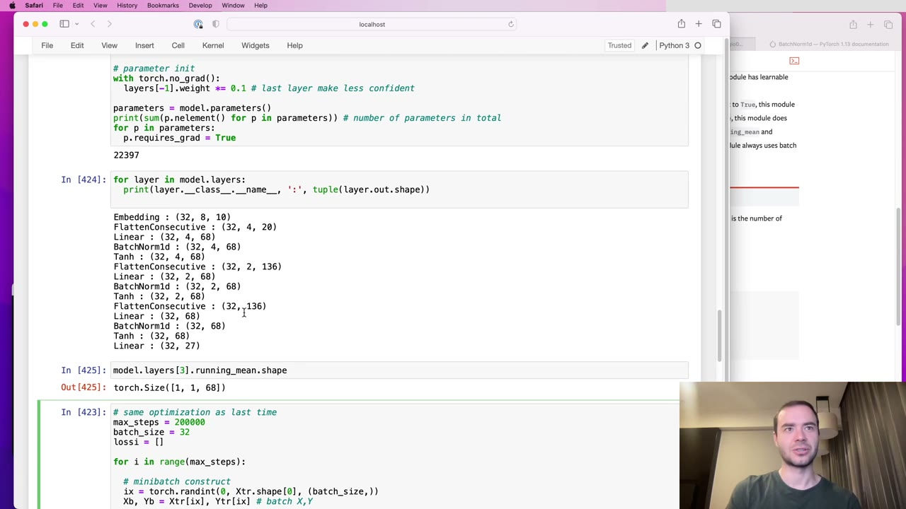
The hierarchical model stacks three blocks of FlattenConsecutive(2), Linear, BatchNorm and tanh (35:06). The first Linear expects n_embd * 2 inputs, the later ones n_hidden * 2. Printing shapes (36:07) shows the tree doing its job: 4 × 8 × 10 becomes 4 × 4 × 20, then 4 × 2 × 400 after the second merge, then 4 × 400 once the last merge squeezes away the single remaining group. The logits come out in the same shape as before.

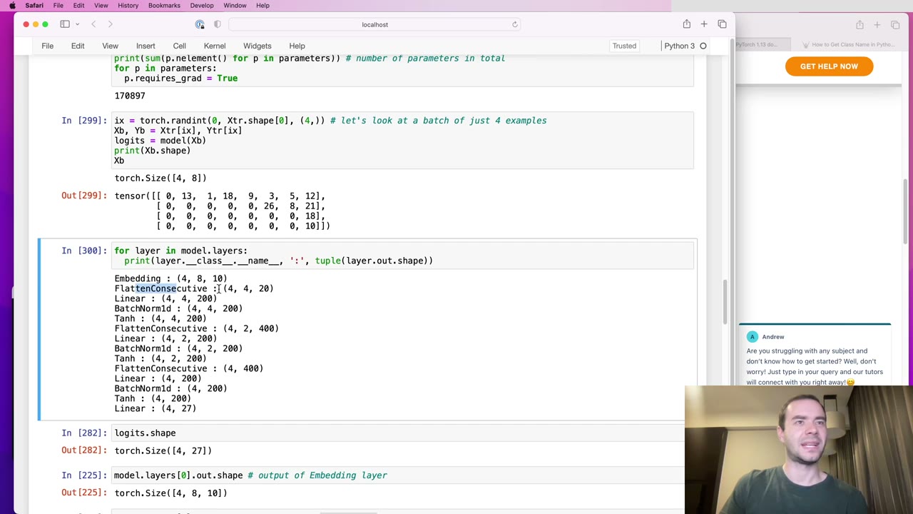
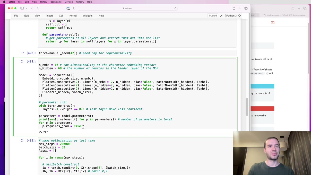
Layer-shape printout for the flat model built with FlattenConsecutive: Embedding (4, 8, 10), FlattenConsecutive (4, 80), Linear (4, 200), BatchNorm1d (4, 200), Tanh (4, 200), Linear (4, 27) — 35:15 — The sanity check: with FlattenConsecutive set to the full block size, the shapes match the old flat model.

Layer-shape printout for the three-level model: Embedding (4, 8, 10), FlattenConsecutive (4, 4, 20), Linear (4, 4, 200), FlattenConsecutive (4, 2, 400), Linear (4, 2, 200), FlattenConsecutive (4, 400), Linear (4, 200), final Linear (4, 27); parameter count 170897 above — 36:20 — The tree in shapes: 4 × 4 × 20, then 4 × 2 × 400, then 4 × 400 at the top. With n_hidden still 200 this version has 170,897 parameters.

This covers one branch of WaveNet’s figure with eight characters of receptive field; the paper’s illustration has four levels and 16 (37:08). To compare fairly, Karpathy sets the hidden size to 68, which brings the parameter count back to about 22,000 (37:40). Result: 2.029 versus 2.027 for the flat model (38:12). He offers two reasons not to give up yet: the channel sizes were a first guess, and BatchNorm might be misbehaving.

Model cell with n_embd = 10, n_hidden = 68 and three FlattenConsecutive(2), Linear(..., bias=False), BatchNorm1d, Tanh blocks, printed parameter count 22397 — 37:48 — Hidden size cut to 68 so the tree model has 22,397 parameters, matching the flat baseline.

split_loss output train 1.9417498111724854, val 2.029465436935425 and performance log adding 'flat → hierarchical (22K params): train 1.941, val 2.029' — 38:10 — Same budget, same loss: the hierarchical model scores 2.029 against 2.027 for the flat one.

38:42 – 46:01 BatchNorm on 3D inputs: the silent bug and the fix

The layer inspector shows BatchNorm receiving 32 × 4 × 68 (38:42). The Part 3 implementation assumed 2D input and took its mean and variance over dimension 0. On a 3D tensor that yields statistics of shape 1 × 4 × 68, and because broadcasting makes all the arithmetic line up, nothing complains (39:45). The running mean confirms it (40:16): the layer is keeping separate statistics for each of the four positions, each estimated from just 32 numbers, when it should keep 68 per-channel statistics computed over 32 × 4 values.

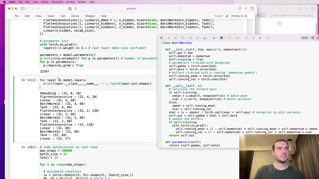
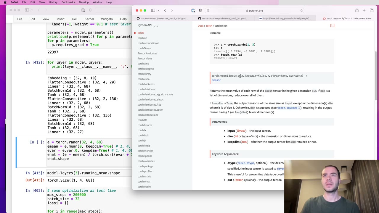
Layer-shape printout for a batch of 32: Embedding (32, 8, 10), FlattenConsecutive (32, 4, 20), Linear (32, 4, 68), BatchNorm1d (32, 4, 68), ... Linear (32, 27), with the BatchNorm1d class shown in an overlay computing x.mean(0, keepdim=True) and x.var(0, keepdim=True) — 38:52 — BatchNorm1d now receives 32 × 4 × 68 tensors, but still reduces over dimension 0 only.

torch.mean accepts a tuple of dimensions (41:51), so the fix is to reduce over (0, 1) when the input is 3D, over 0 when it’s 2D, and any other input now fails with an error (42:54). The running statistics become 1 × 1 × 68.

PyTorch documentation for torch.mean(input, dim, keepdim=False, *, dtype=None, out=None), where dim is 'the dimension or dimensions to reduce', open over the layer-shape printout — 41:53 — torch.mean accepts a tuple of dimensions, which makes the fix a one-line change.

Cell e = torch.randn(32, 4, 68); emean = e.mean((0,1), keepdim=True); evar = e.var((0,1), keepdim=True); ehat.shape = torch.Size([32, 4, 68]); emean.shape = torch.Size([1, 1, 68]); model.layers[3].running_mean.shape = torch.Size([1, 4, 68]) — 42:35 — Reducing over (0, 1) gives one statistic per channel (1 × 1 × 68); the current layer's running mean is still 1 × 4 × 68.

Edited BatchNorm1d.__call__: if x.ndim == 2: dim = 0; elif x.ndim == 3: dim = (0,1); xmean = x.mean(dim, keepdim=True); xvar = x.var(dim, keepdim=True) — 43:38 — The fixed BatchNorm1d: the reduction dimensions depend on whether the input is 2D or 3D.

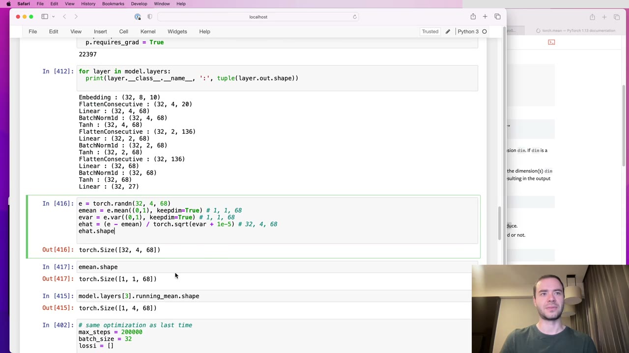
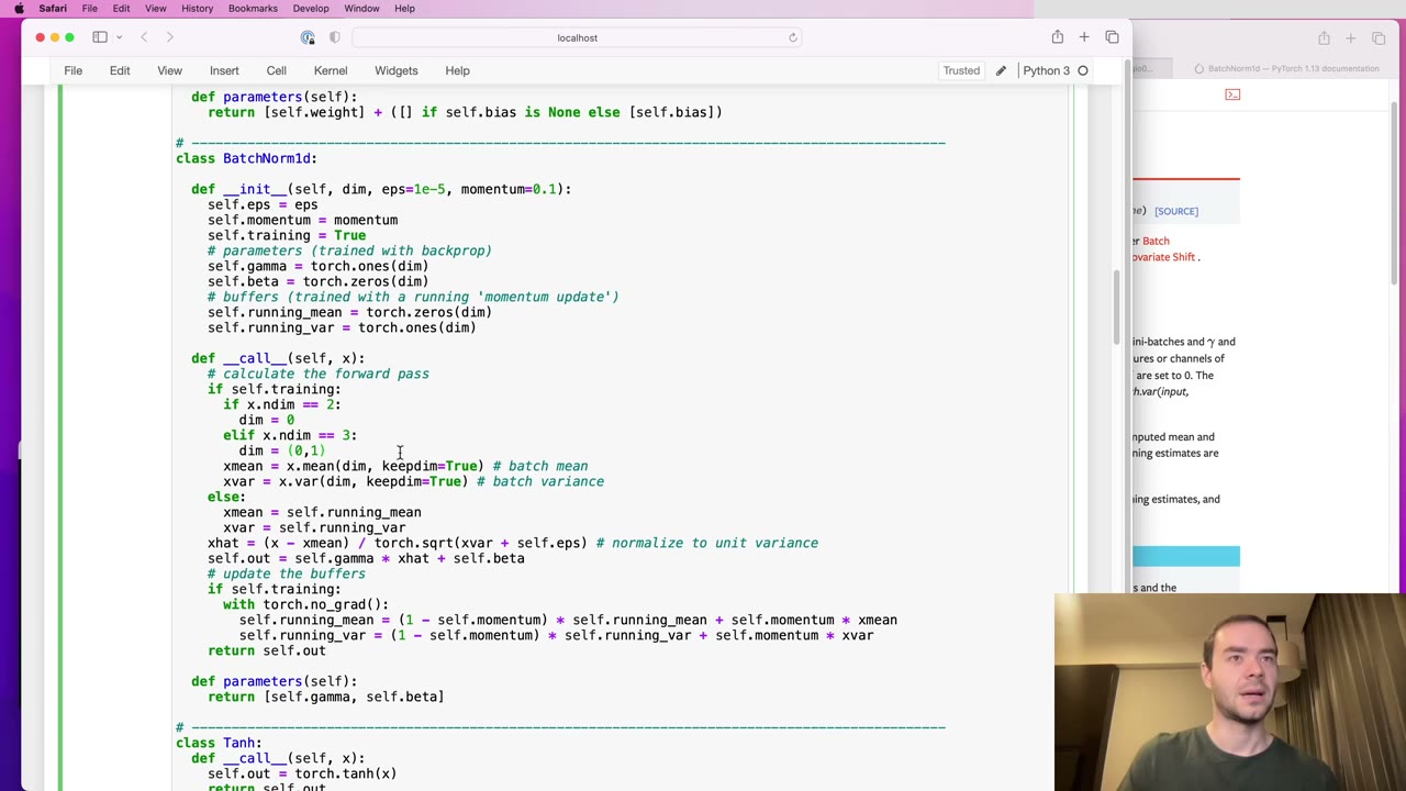
Karpathy flags that this departs from PyTorch (43:24). torch.nn.BatchNorm1d accepts 3D input only as N × C × L, with channels in the middle, and reduces over dimensions 0 and 2. His version assumes channels come last, N × L × C, and he says he prefers it that way. Retraining gives 2.022 (44:57), a small gain he won’t call significant. He expected some improvement, since each statistic now rests on four times as many numbers and is less noisy.

PyTorch BatchNorm1d documentation, Shape section: Input (N, C) or (N, C, L), where N is the batch size, C the number of features or channels, L the sequence length; Output same shape as input — 43:50 — PyTorch's BatchNorm1d expects channels in the middle (N, C, L); the lecture's version assumes channels last.

Layer-shape printout after the fix and model.layers[3].running_mean.shape returning torch.Size([1, 1, 68]) — 45:04 — After the fix the running mean has one entry per channel.

split_loss output train 1.9123165607452393, val 2.022149085998535 and performance log adding 'fix bug in batchnorm: train 1.912, val 2.022' — 45:25 — Retraining with the fixed layer: validation 2.022, a small improvement.

Our note: if you swap in torch.nn.BatchNorm1d later, you need to transpose to (N, C, L) before the layer and back afterwards, or the normalization runs over the wrong axis.

46:01 – 47:33 Scaling up to 1.993, with caveats

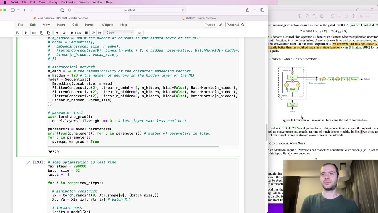
With the architecture now general, Karpathy widens it: embeddings of 24 dimensions instead of 10 and 128 hidden units instead of 68, 76,579 parameters in total (46:01). Validation loss reaches 1.993, the first result under 2.0. Training now takes noticeably longer, and he is frank that the tuning is guesswork (46:31): there is no experiment harness, only the training loss is being watched closely, and the hyperparameters are unsearched. He also lists what was left out of WaveNet: the gated activation, residual connections and skip connections (47:02).

Model cell with n_embd = 24, n_hidden = 128, three FlattenConsecutive(2), Linear(..., bias=False), BatchNorm1d(n_hidden), Tanh() blocks and Linear(n_hidden, vocab_size); printed parameter count 76579 — 46:12 — The scaled-up network: 24-dimensional embeddings, 128 hidden units, 76,579 parameters.

split_loss output train 1.7690284252166748, val 1.9936515092849731 and the full performance log ending with 'scale up the network: n_embd 24, n_hidden 128 (76K params): train 1.769, val 1.993' — 46:30 — The final result, 1.993, and the full performance log of the lecture.

WaveNet paper section 2.4, Residual and skip connections, Figure 4 overview of the residual block with dilated conv, tanh and sigmoid gates, 1x1 convolutions and skip connections, next to the performance log — 47:29 — The parts of WaveNet left out: gated activations, residual and skip connections.

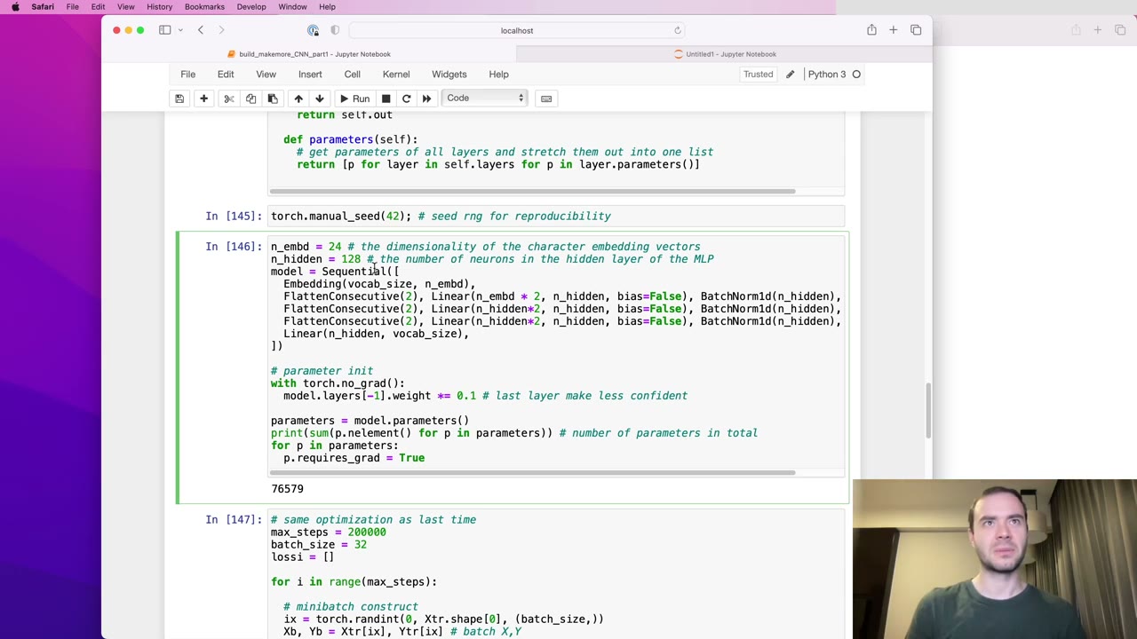
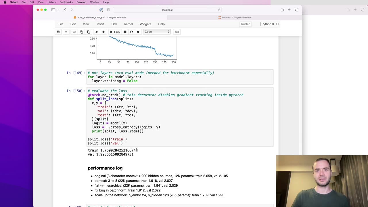
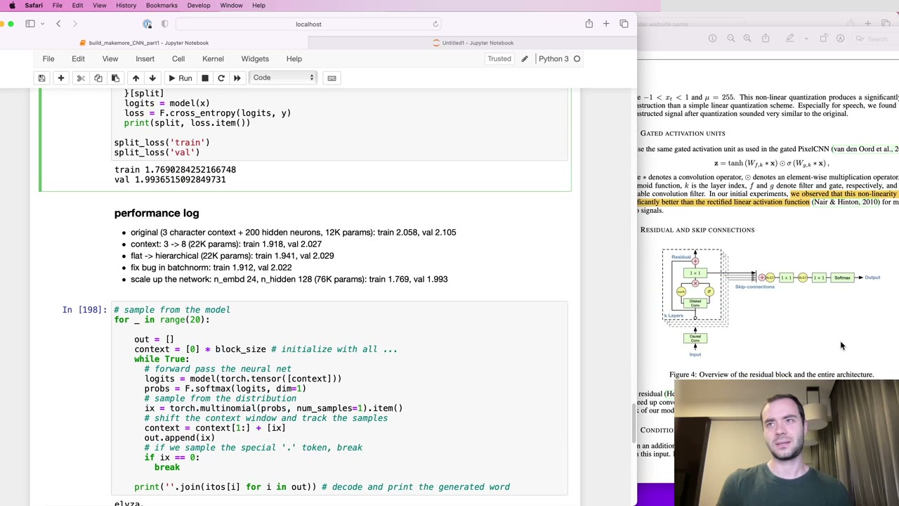
Our note: the published notebook in nn-zero-to-hero uses n_embd = 24 and n_hidden = 128 for this final run.

47:33 – 51:42 Where convolutions come in

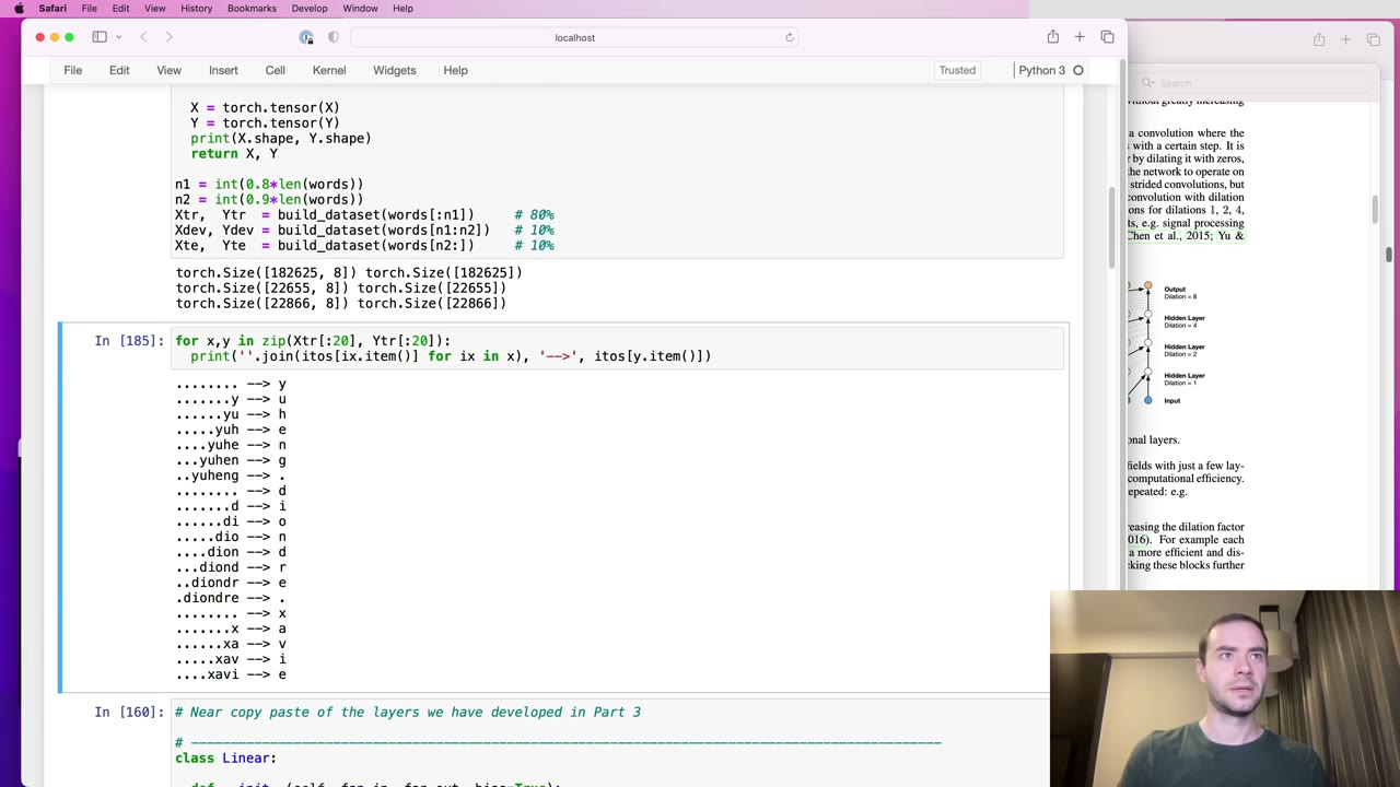
The closing preview explains WaveNet’s convolutions without implementing them. Take one name from the training set, “diondre”: its seven letters yield eight separate training examples, one per position (48:05). You could forward each one with its own call (adding a batch dimension of one), or loop over all eight and fill a preallocated output. Either way it’s eight independent passes through the tree.

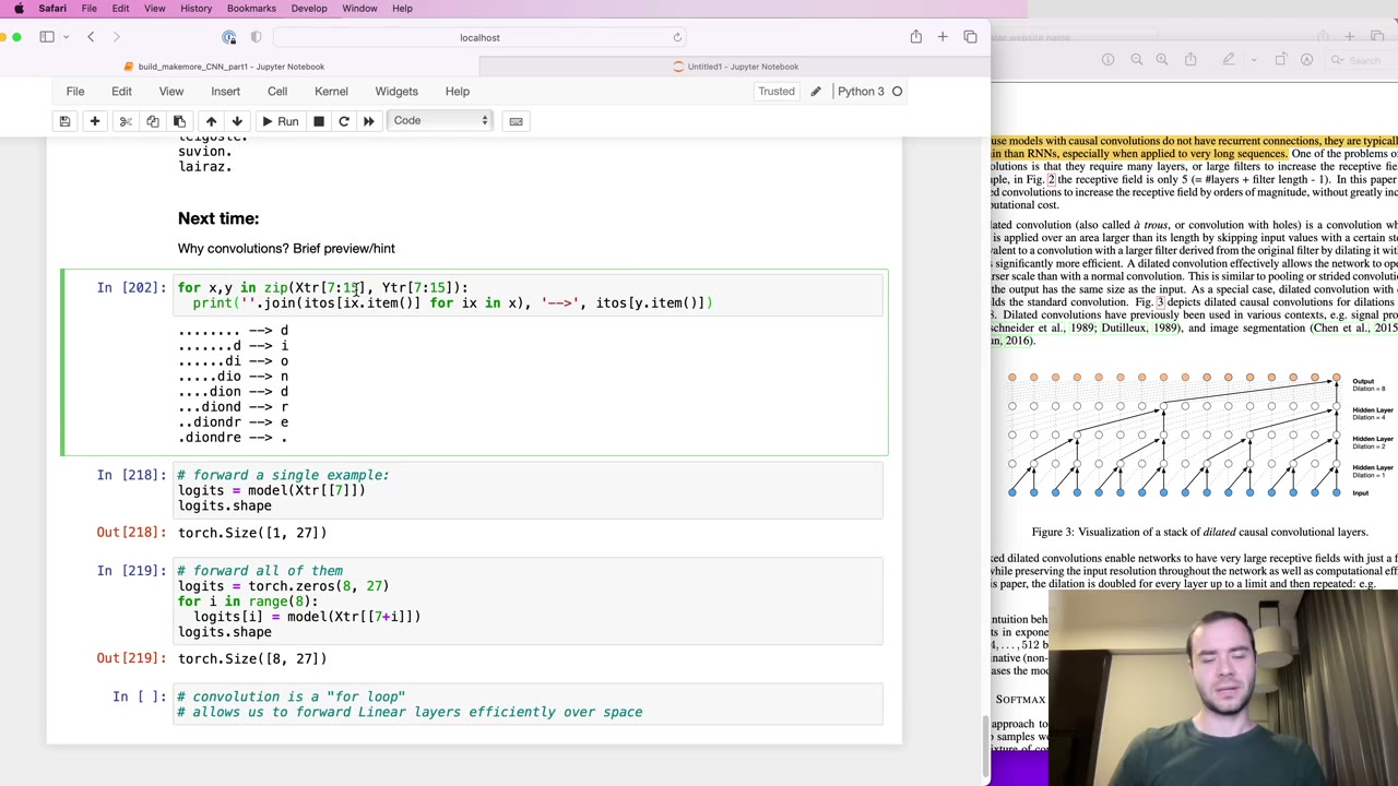
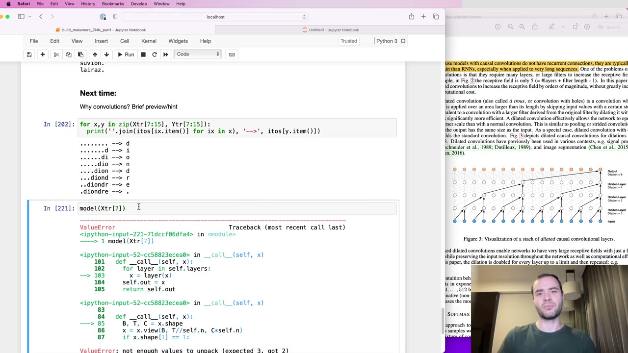
Cell printing Xtr[7:15] as eight examples of the name diondre (........ → d up to .diondre → .), then logits = model(Xtr[[7]]) with shape torch.Size([1, 27]) and a loop filling logits = torch.zeros(8, 27) with shape torch.Size([8, 27]), beside WaveNet's Figure 3 — 48:02 — One name, diondre, gives eight examples; forwarding them one at a time is a Python loop.

Cell model(Xtr[7]) raising ValueError in FlattenConsecutive.__call__ at B, T, C = x.shape: not enough values to unpack (expected 3, got 2) — 48:40 — Without the extra batch dimension the model fails: Xtr[7] is a 1D row of eight, so FlattenConsecutive can't unpack three dimensions.

A convolution does that loop for you (49:07). It slides the same small linear filter along the sequence, and the loop runs inside CUDA kernels rather than in Python. The second benefit is reuse (50:41). In the tree diagram, an intermediate node can be the right child of one parent and the left child of the next, so neighbouring outputs share work. Computed one example at a time, that node is recalculated; in the convolutional version it’s computed once. The Linear layers become filters slid over the sequence, layer by layer. Karpathy defers the implementation to a future video.

Our note: in the WaveNet paper the dilation doubles at each layer (1, 2, 4, 8), which is the convolutional way of saying “merge pairs, then pairs of pairs”, the same tree as FlattenConsecutive(2) stacked three times.

51:42 – 54:16 torch.nn is unlocked, and what the workflow looks like

Karpathy steps back (51:42). Over these lectures the class has rebuilt a small version of torch.nn on top of torch.Tensor: layers, containers and parameters. He considers it unlocked, and from here on the series will use the real library.

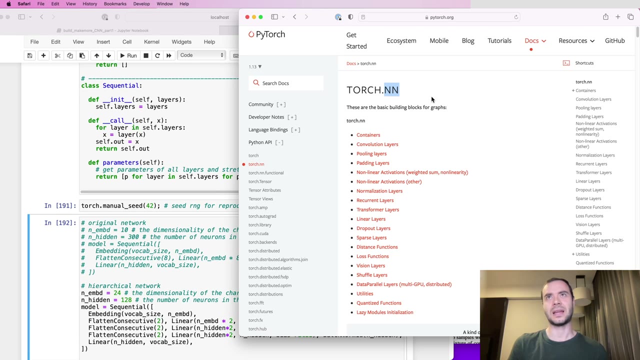
PyTorch documentation page for torch.nn listing Containers, Convolution Layers, Pooling layers, Normalization Layers and other module groups, over the notebook's Sequential class and model cell — 52:01 — The torch.nn index: the class has now rebuilt small versions of its containers and layers by hand.

He then describes his development process as fairly representative (52:13):

A lot of time goes into the PyTorch documentation, which he criticises sharply (52:44): in his view it can be wrong, incomplete or unclear.
Much of the work is shape gymnastics: 2D, 3D or 4D, NCL or NLC, views and reshapes (53:14).
He prototypes layers in a Jupyter notebook until the shapes check out, then pastes the code into a repository in VS Code and launches experiments from there (53:44).

54:16 – end What’s next, and a challenge

The list of follow-ups (54:16): implement the dilated causal convolutions, explain residual and skip connections, set up a real experiment harness with many runs, plots and hyperparameter searches (54:47), and cover RNNs, LSTMs, GRUs and Transformers. In a postscript (55:19) he invites viewers to beat 1.993: reallocate channels, change the embedding size, read the WaveNet paper and implement its layers, tune initialization or optimization. He adds a pointed possibility (55:49): a single-hidden-layer network made big enough might beat the “fancy” hierarchical one.

Final notebook model cell with the commented-out original network and the hierarchical network (n_embd = 24, n_hidden = 128), parameter count 76579, beside the WaveNet paper's residual-block figure — 54:31 — Where the notebook ends: the hierarchical model at 76,579 parameters, with WaveNet's residual and skip connections still to come.

Code you’ll write

These are short excerpts in the style of the lecture notebook. The full notebook (makemore_part5_cnn1.ipynb) is in karpathy/nn-zero-to-hero, MIT-licensed, and the standalone makemore script is in karpathy/makemore.

1. Embedding and Sequential modules. Moves the embedding lookup into a layer and wraps all layers in one container, built at 10:24 and 13:33.

class Embedding:
  def __init__(self, num_embeddings, embedding_dim):
    self.weight = torch.randn((num_embeddings, embedding_dim))
  def __call__(self, IX):
    self.out = self.weight[IX]
    return self.out
  def parameters(self):
    return [self.weight]

class Sequential:
  def __init__(self, layers):
    self.layers = layers
  def __call__(self, x):
    for layer in self.layers:
      x = layer(x)
    self.out = x
    return self.out
  def parameters(self):
    return [p for layer in self.layers for p in layer.parameters()]

2. FlattenConsecutive. Concatenates every n neighbouring vectors and turns the groups into a batch dimension, written at 31:24.

class FlattenConsecutive:
  def __init__(self, n):
    self.n = n
  def __call__(self, x):
    B, T, C = x.shape
    x = x.view(B, T//self.n, C*self.n)
    if x.shape[1] == 1:
      x = x.squeeze(1)
    self.out = x
    return self.out
  def parameters(self):
    return []

3. BatchNorm1d that handles 3D input. The changed part of the forward pass: reduce over the batch and the group dimension, as fixed at 42:54.

  def __call__(self, x):
    if self.training:
      if x.ndim == 2:
        dim = 0
      elif x.ndim == 3:
        dim = (0, 1)
      xmean = x.mean(dim, keepdim=True)  # batch mean
      xvar = x.var(dim, keepdim=True)    # batch variance
    else:
      xmean = self.running_mean
      xvar = self.running_var
    xhat = (x - xmean) / torch.sqrt(xvar + self.eps)
    self.out = self.gamma * xhat + self.beta
    # ...running_mean / running_var updates unchanged

4. The hierarchical model. Three merge levels over a block_size of 8, assembled at 35:06 and scaled up at 46:01.

n_embd = 24    # embedding size per character
n_hidden = 128 # neurons per hidden layer
model = Sequential([
  Embedding(vocab_size, n_embd),
  FlattenConsecutive(2), Linear(n_embd * 2, n_hidden, bias=False), BatchNorm1d(n_hidden), Tanh(),
  FlattenConsecutive(2), Linear(n_hidden * 2, n_hidden, bias=False), BatchNorm1d(n_hidden), Tanh(),
  FlattenConsecutive(2), Linear(n_hidden * 2, n_hidden, bias=False), BatchNorm1d(n_hidden), Tanh(),
  Linear(n_hidden, vocab_size),
])
with torch.no_grad():
  model.layers[-1].weight *= 0.1  # less confident at init
parameters = model.parameters()
for p in parameters:
  p.requires_grad = True

5. Smoothing the loss plot and switching to eval mode. Averages blocks of 1,000 steps (8:21) and turns off BatchNorm’s training behaviour before evaluating or sampling (15:44).

plt.plot(torch.tensor(lossi).view(-1, 1000).mean(1))

for layer in model.layers:
  layer.training = False

Skip list

1:35 – 5:15 Starter-code recap. Skip if you’ve just finished makemore Part 3; the one new detail is the global RNG seed.
12:32 – 13:03 A microphone change and the lead-in to containers.
20:22 – 21:27 Waiting on the flat block-size-8 baseline; the number (about 2.02) is all you need.
28:45 – 29:49 The explicit even/odd concatenation, if you’re comfortable with view; it exists to prove that the one-line reshape is equivalent.
52:44 – 53:14 The aside about PyTorch’s documentation.

Glossary

WaveNet — a 2016 DeepMind model for generating audio one sample at a time, whose stacked layers merge the context in a tree; this lecture borrows only that tree shape.
Autoregressive model — a model that predicts the next element of a sequence from the elements before it, then feeds its own prediction back in to keep going.
block_size — how many previous characters the model sees; raised from 3 to 8 here.
Receptive field — the span of input positions that can influence one output; eight characters for this three-level tree.
n_embd / n_hidden — the size of each character’s embedding vector and the width of each hidden layer.
Embedding layer — a learned lookup table that maps each character index to a vector.
Batch dimension — any leading tensor dimension that an operation processes in parallel; here both the examples and the character groups play this role.
view — a PyTorch reshape that changes how a tensor’s memory is read without copying it.
FlattenConsecutive — Karpathy’s layer that merges every n adjacent vectors into one and keeps the groups as a batch dimension.
Sequential — a container module that runs layers one after another and gathers their parameters.
Running statistics — BatchNorm’s moving averages of mean and variance, used instead of batch statistics at evaluation time.
Training / evaluation mode — the flag that tells stateful layers such as BatchNorm which behaviour to use; forgetting to switch it causes silent errors.
NCL vs NLC — two layouts for sequence tensors: channels in the middle (PyTorch’s BatchNorm1d) or channels last (this lecture’s version).
Dilated causal convolution — a convolution that only looks backward in time and skips positions at growing intervals, so stacked layers cover a long context; WaveNet’s efficient form of the tree.

FAQ

What is the WaveNet-style architecture built in makemore Part 5?

Instead of concatenating all eight context characters and pushing them through one hidden layer, the model fuses them in a tree. The first layer combines neighbouring pairs of characters, the second combines pairs of those pairs, and the third combines the two remaining halves, so information is merged gradually as the network gets deeper. Karpathy borrows the idea from the 2016 WaveNet paper from DeepMind, but implements only this hierarchical structure, not WaveNet's gated activations, residual or skip connections.

What does FlattenConsecutive do, and why not use torch.nn.Flatten?

FlattenConsecutive(n) takes a tensor shaped (B, T, C) and views it as (B, T//n, C*n), so every n neighbouring vectors are concatenated into one longer vector while the remaining groups become an extra batch dimension. If only one group is left, it squeezes that dimension away. Karpathy gives it a new name because PyTorch's own Flatten takes different arguments and behaves differently, and he did not want his layer to pretend to match it.

Why did BatchNorm1d need fixing when the input became three-dimensional?

The original layer computed its mean and variance over dimension 0 only. With a 32 by 4 by 68 input that silently produced statistics of shape 1 by 4 by 68, so the layer kept separate running statistics for each of the four positions, each estimated from just 32 numbers. Nothing errored because broadcasting made the arithmetic work. The fix is to reduce over dimensions (0, 1) when the input is 3D, giving one mean and variance per channel. Validation loss improved slightly, from 2.029 to 2.022.

Does the hierarchical model actually beat the flat MLP?

Not at first. With the parameter count held at about 22,000, the tree model scored 2.029 against 2.027 for the flat MLP with the same eight-character context. After the BatchNorm fix it reached 2.022, and only after widening the embeddings to 24 dimensions and the hidden layers (about 76,000 parameters) did it get to 1.993. Karpathy says himself that these numbers come from guess-and-check without a proper experiment harness.

Does this lecture implement convolutions?

No. The final segment explains how the model relates to the dilated causal convolutions in WaveNet: a convolution slides the same tree over every position of a sequence inside a CUDA kernel and reuses intermediate nodes that neighbouring outputs share. The lecture computes one output at a time, and Karpathy leaves the convolutional version for a future video.

Studying another course? Paste its YouTube or Bilibili link on the home page to request a handout — or make your own with the desktop app (coming soon).