Karpathy's Zero to Hero, Lecture 3: makemore Part 2, the MLP — notes, code and timestamps
 1:50
 3:01
 4:22
 5:49
 9:05
 9:51
 11:39
 11:57
 13:29
 14:43
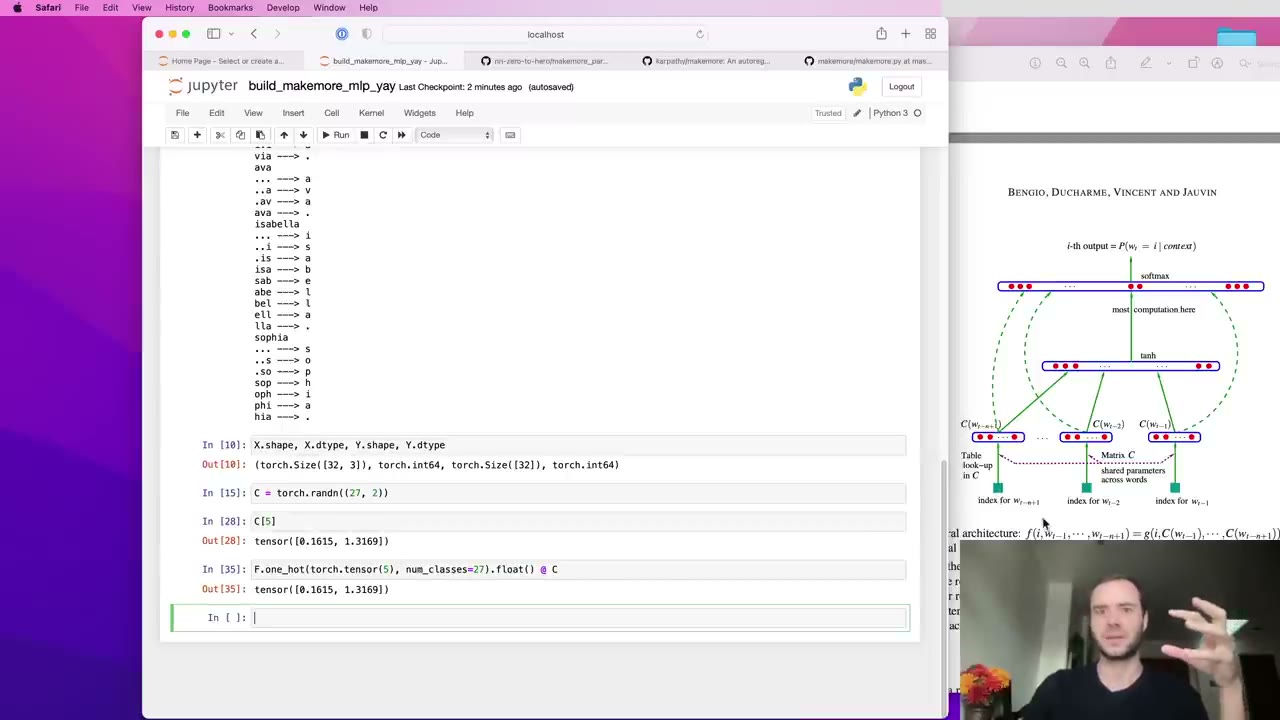 15:45
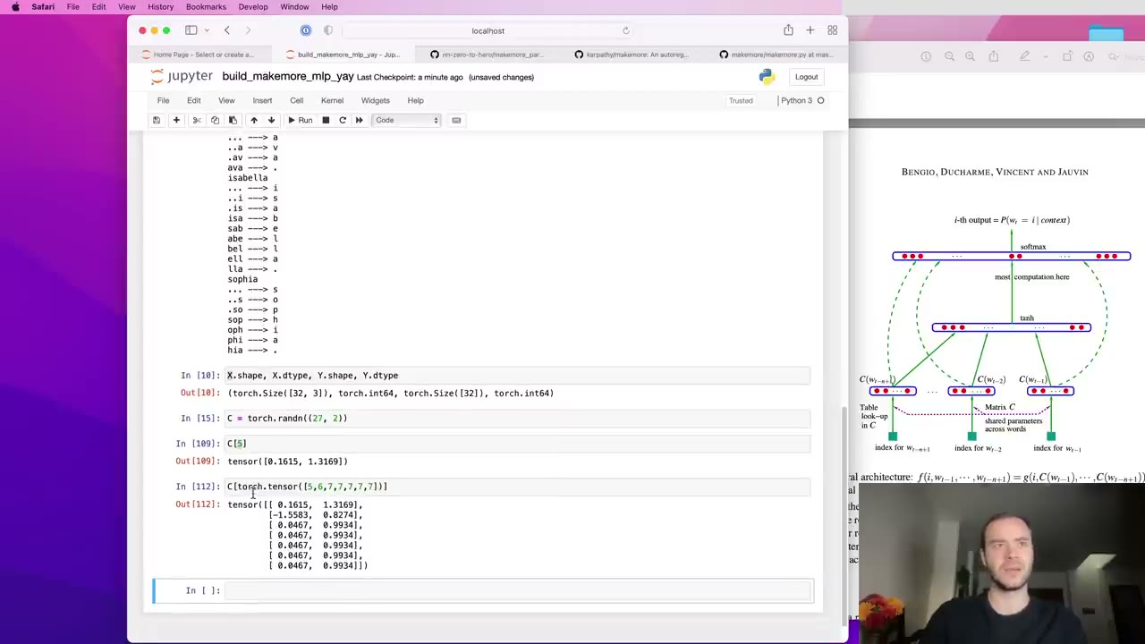 17:16
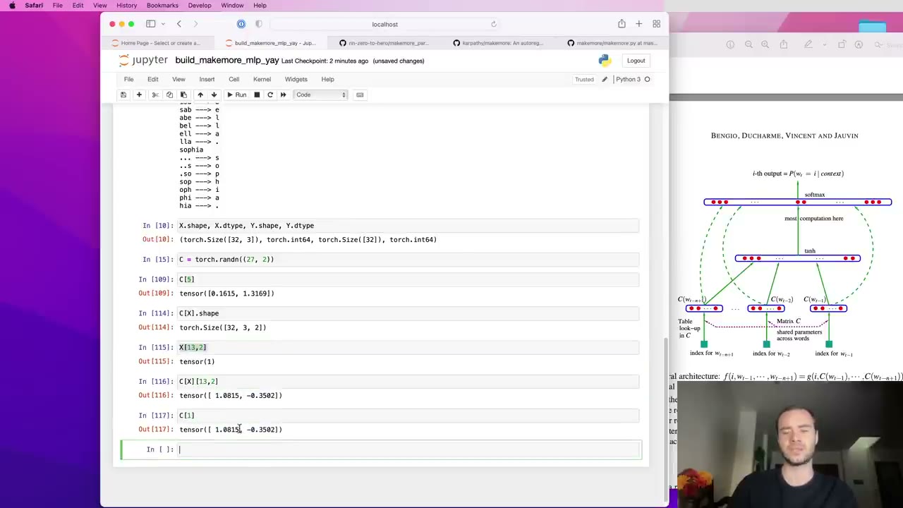 18:20
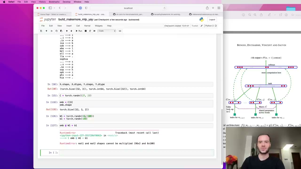 19:44
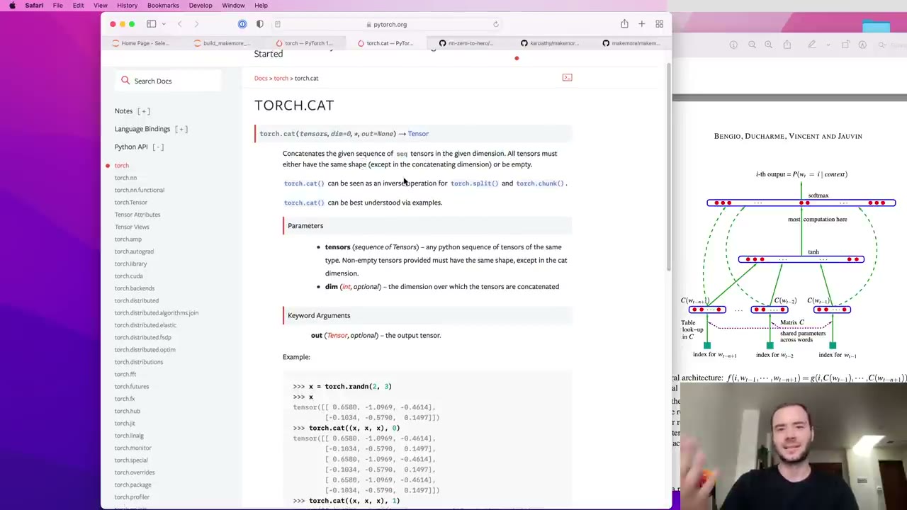 20:49
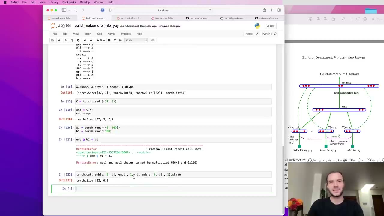 22:12
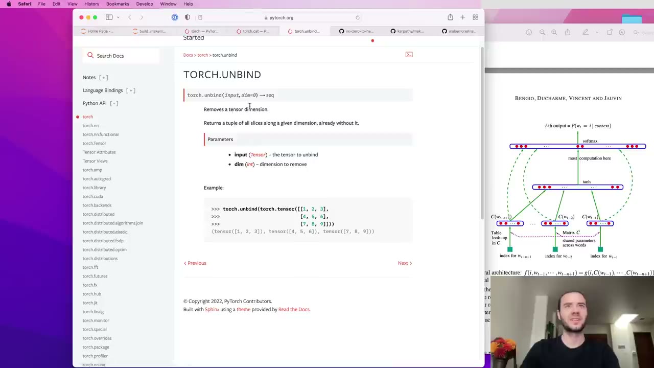 22:36
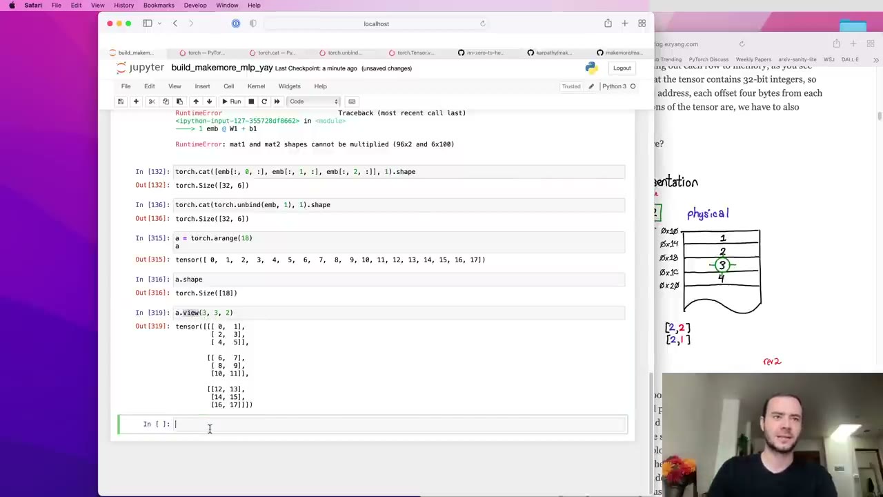 24:25
 25:31
 26:26
 28:22
 28:35
 29:50
 31:47
 32:18
 33:32
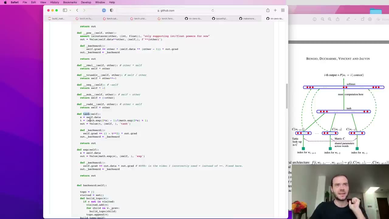 34:21
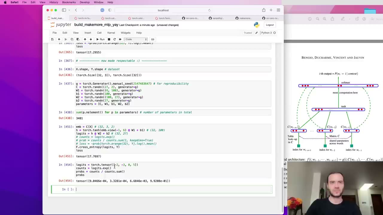 35:28
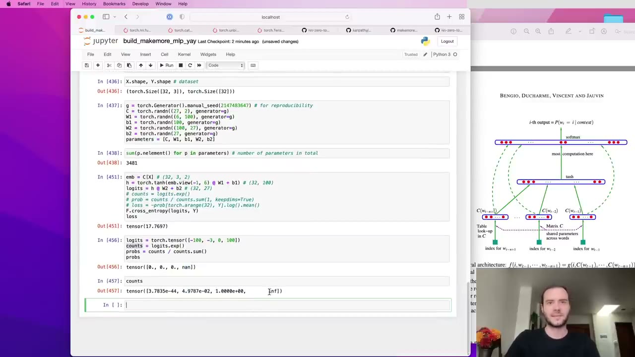 36:09
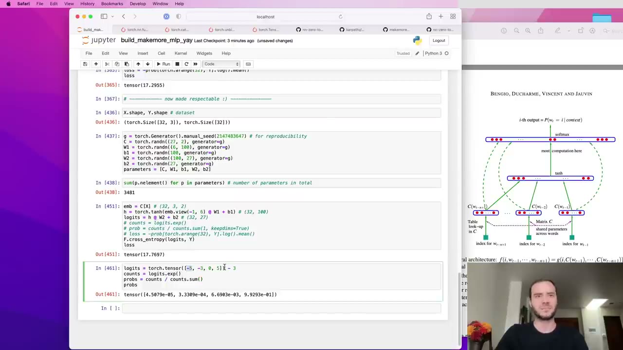 37:15
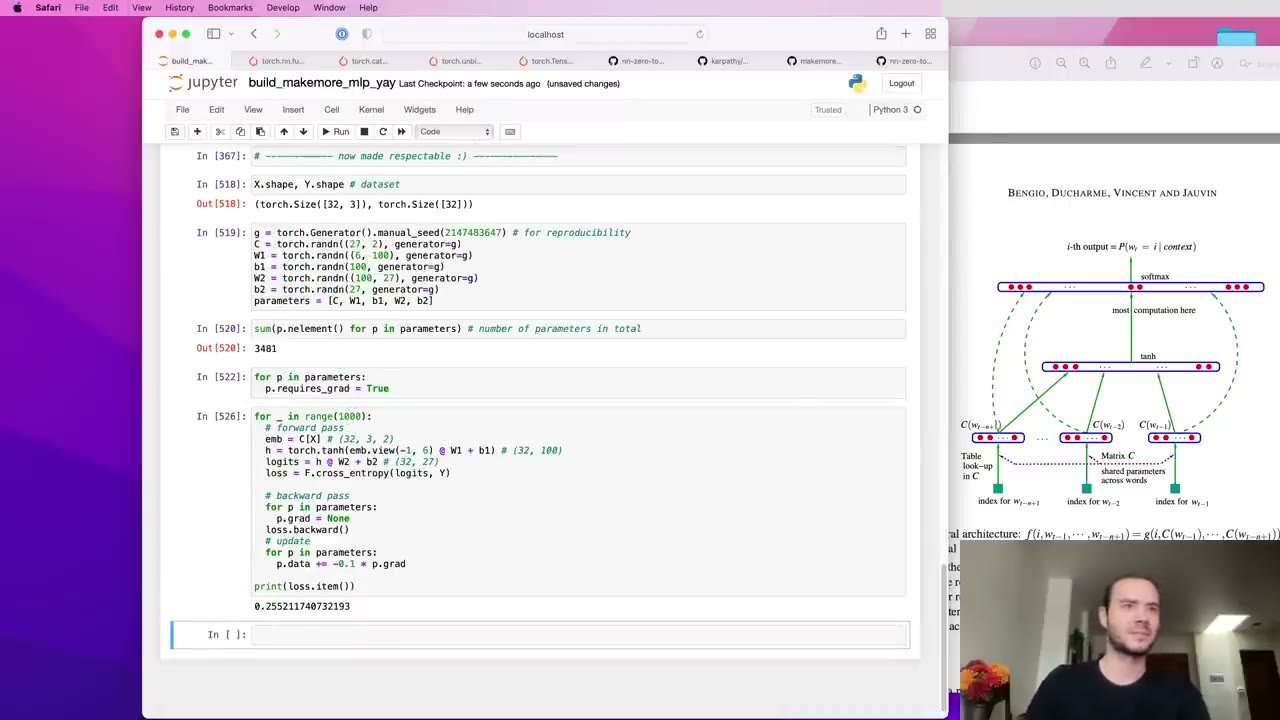 39:19
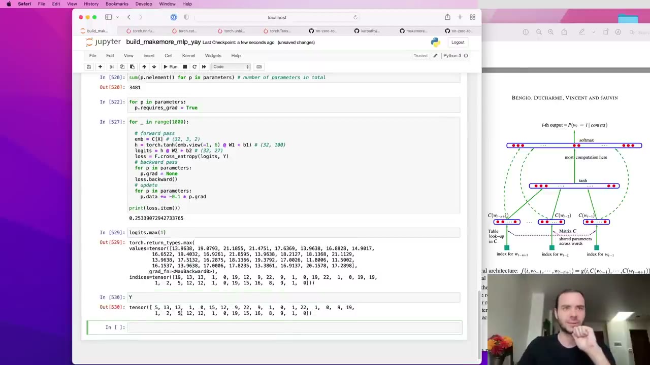 40:25
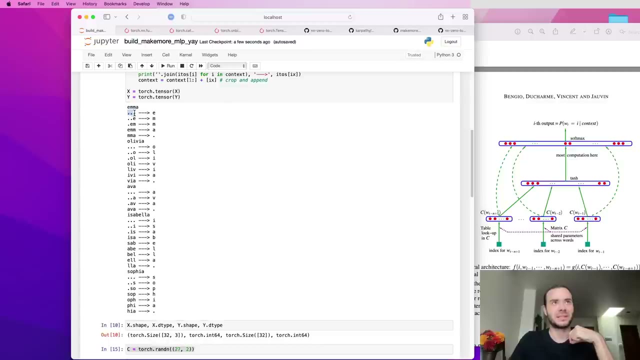 40:44
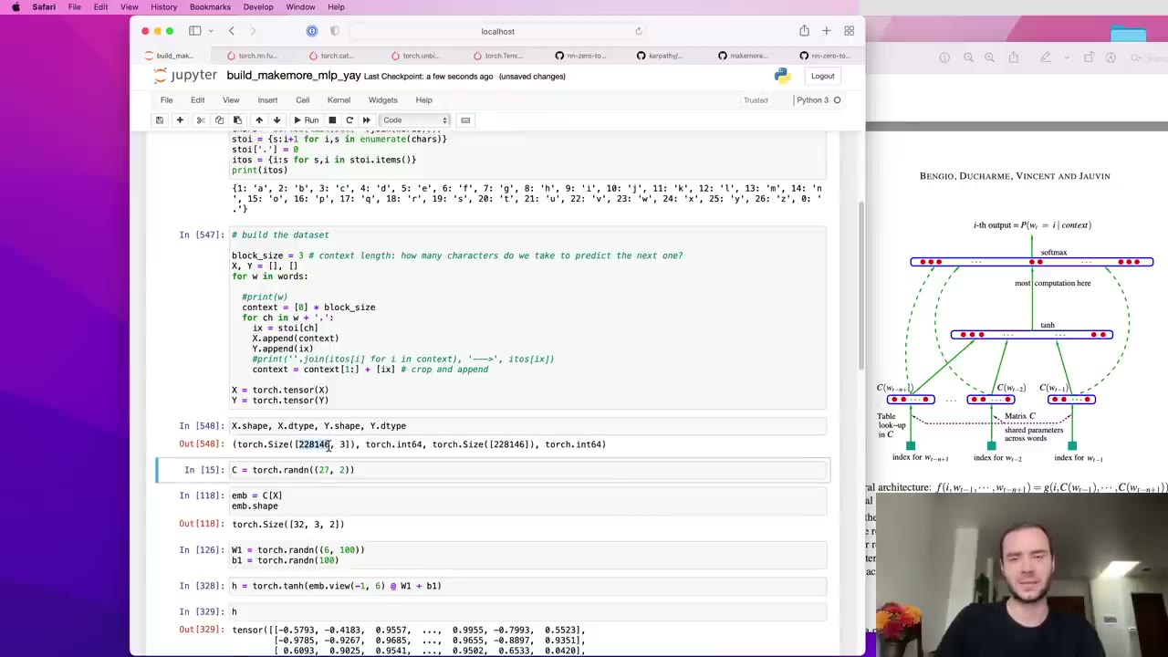 41:43
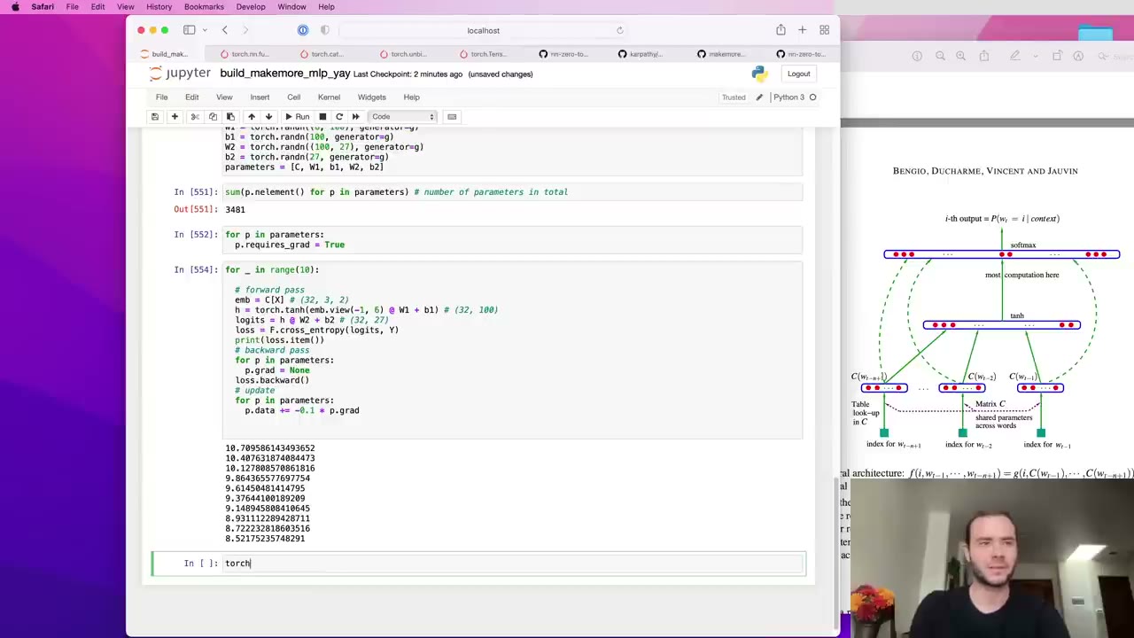 42:43
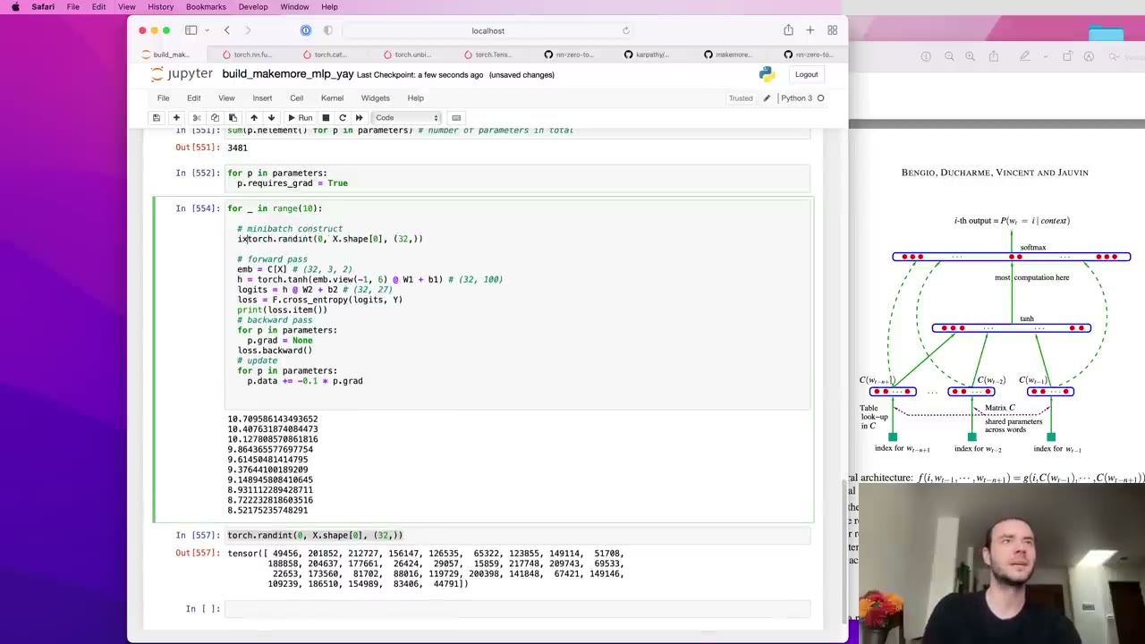 43:20
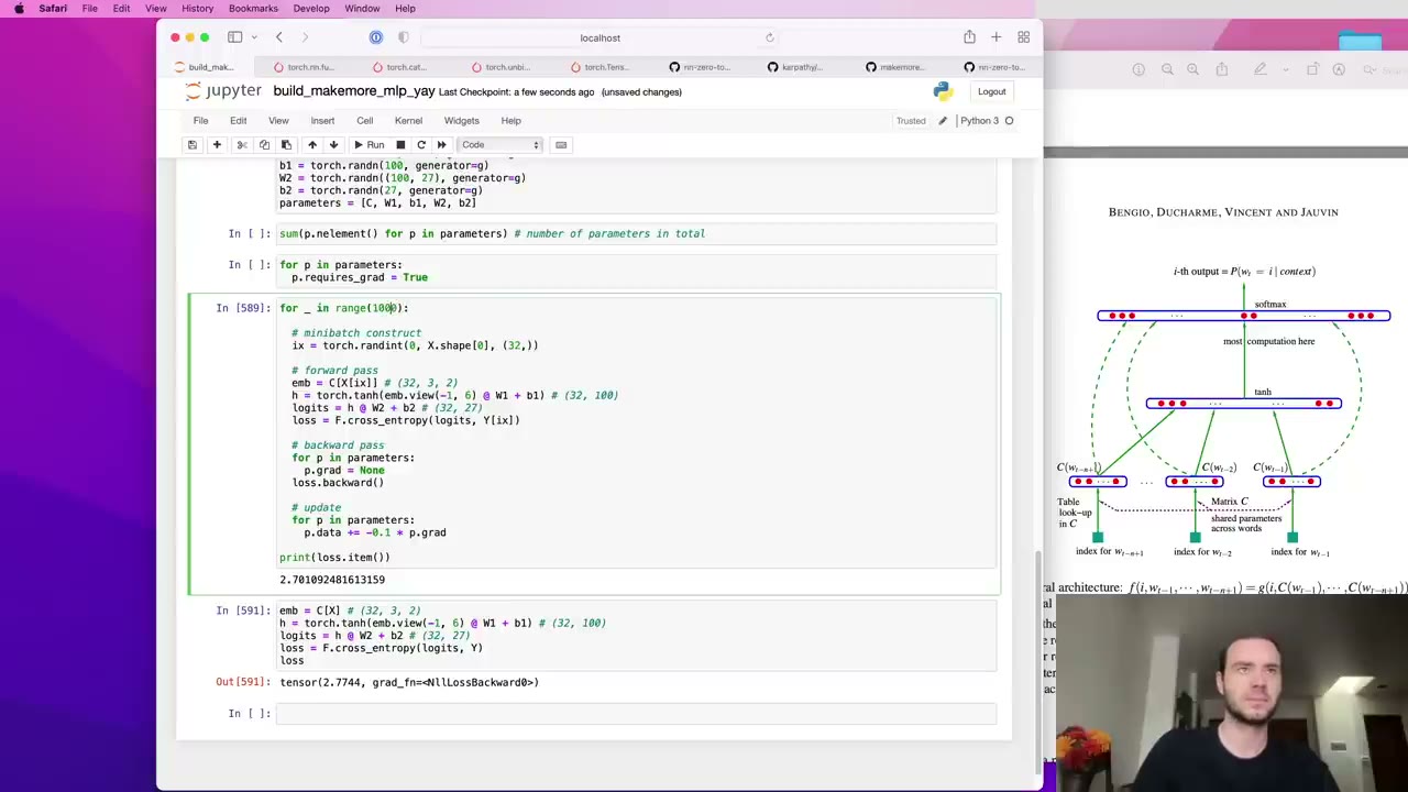 45:10
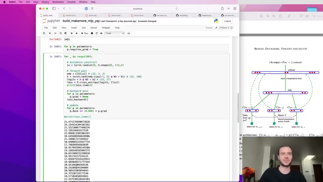 46:14
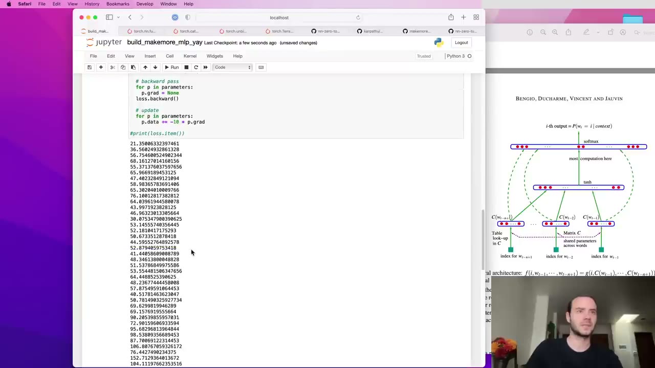 46:46
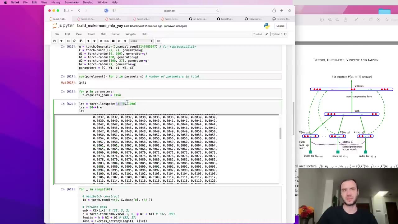 47:52
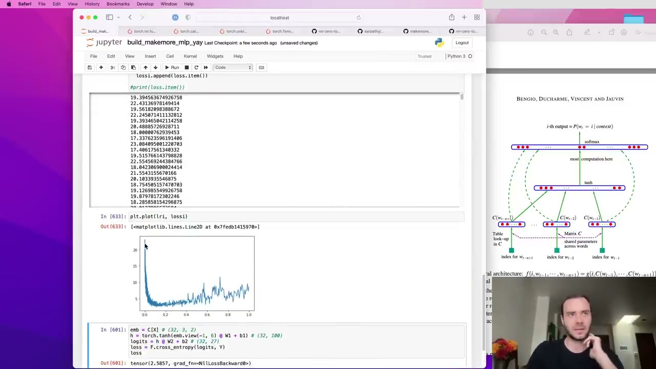 49:50
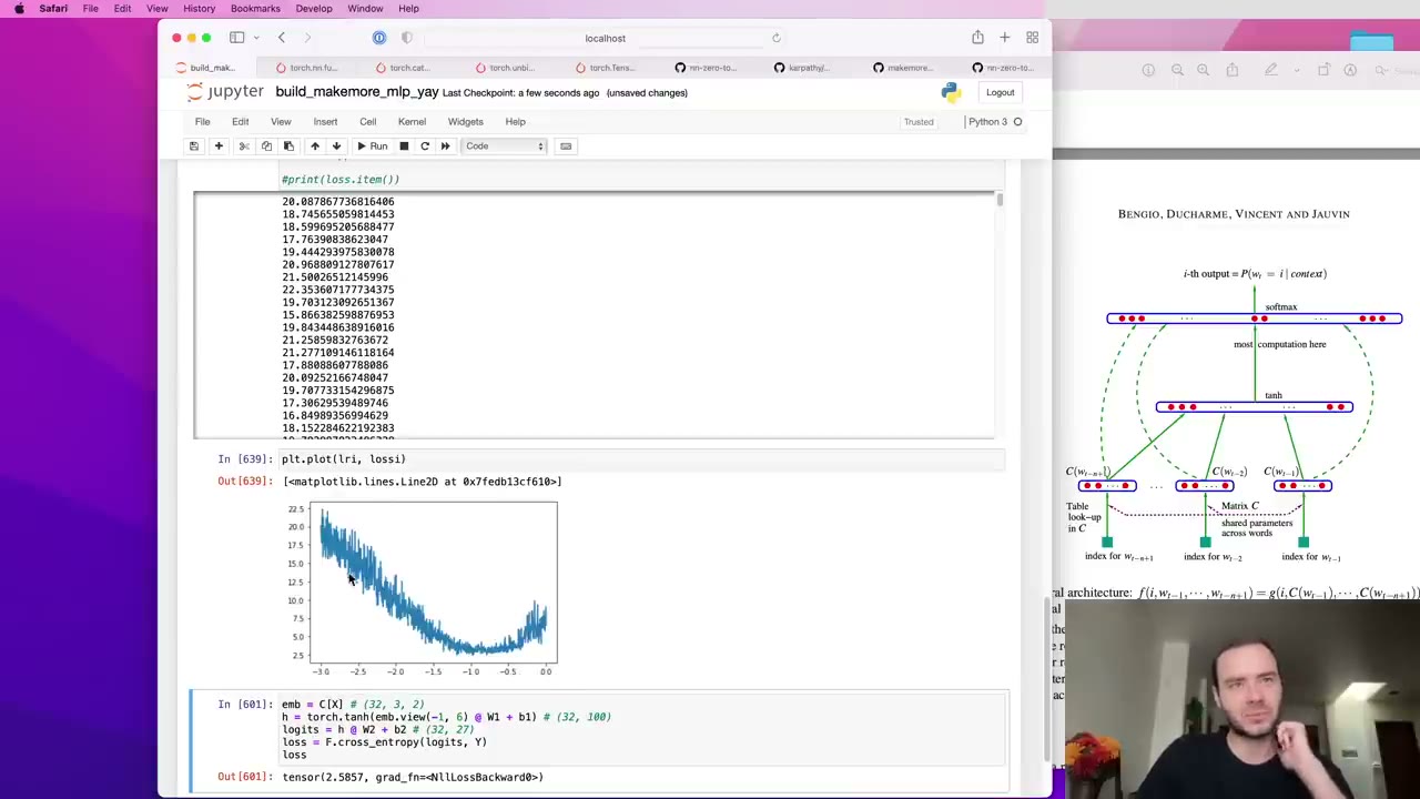 50:37
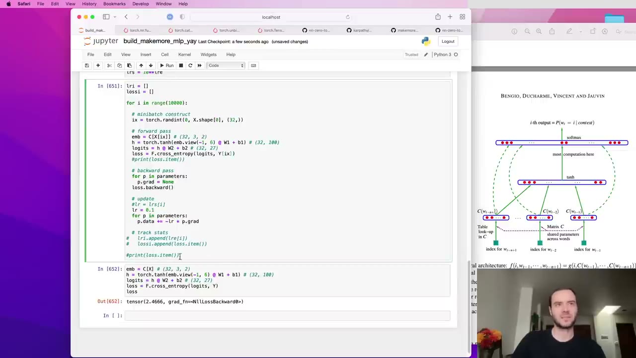 52:01
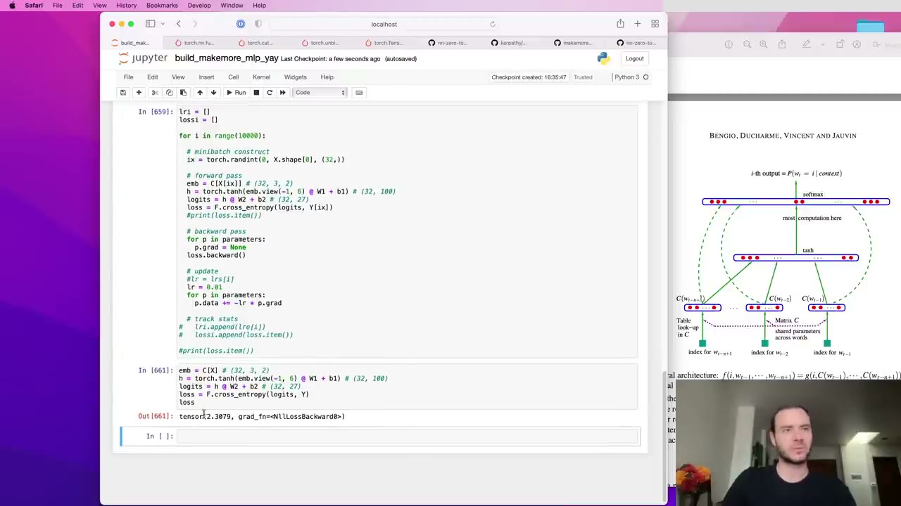 53:09
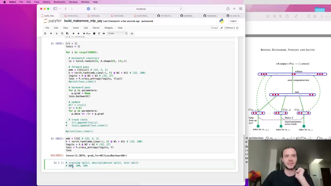 55:05
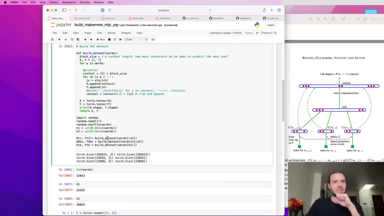 57:29
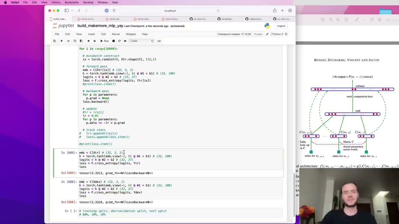 1:00:28
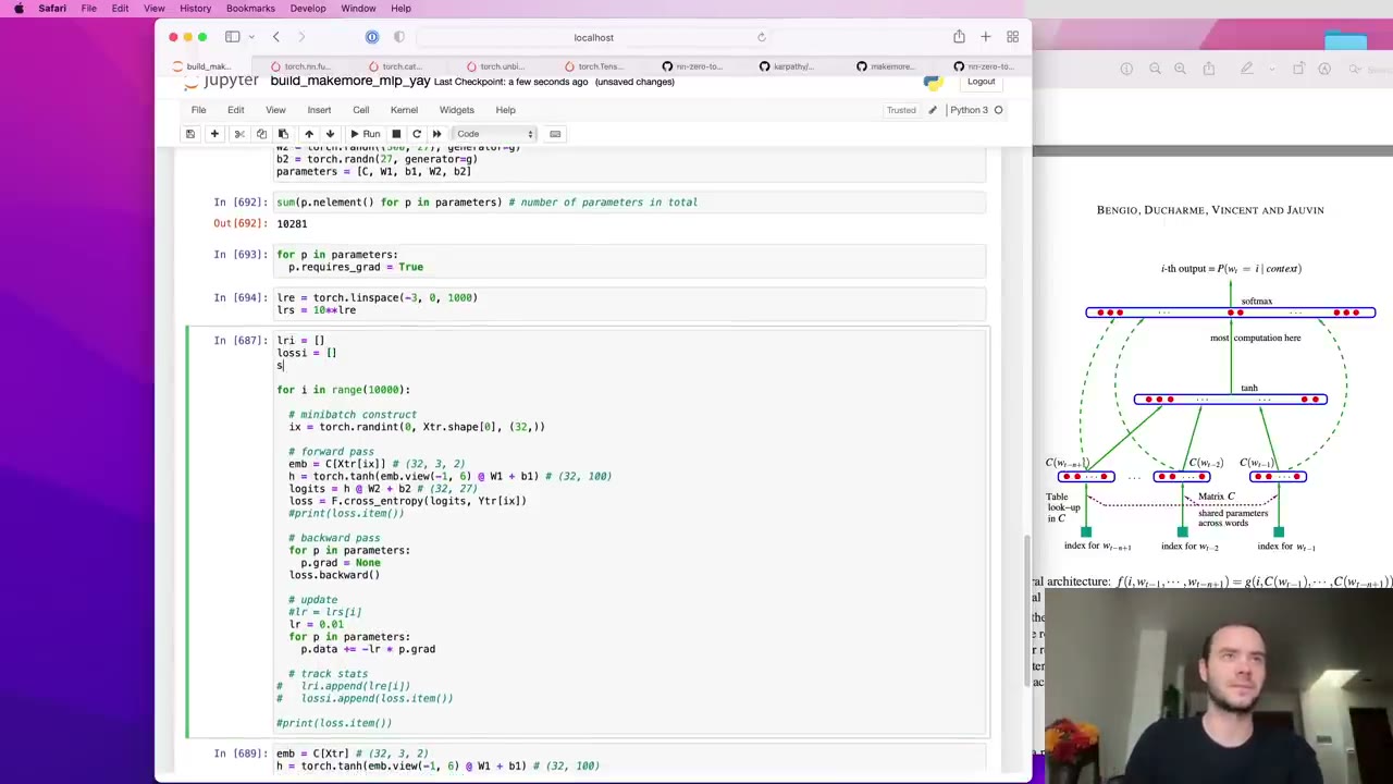 1:01:22
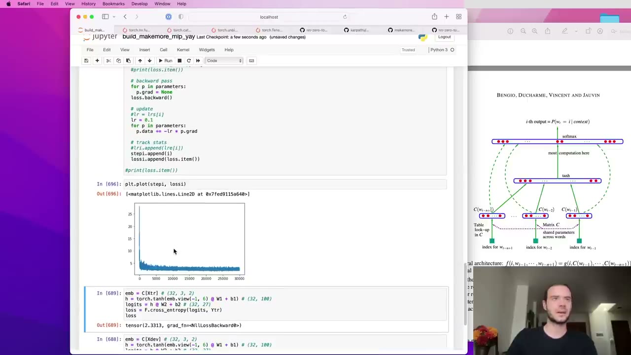 1:02:15
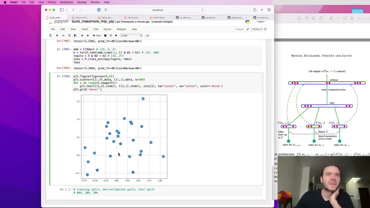 1:06:02
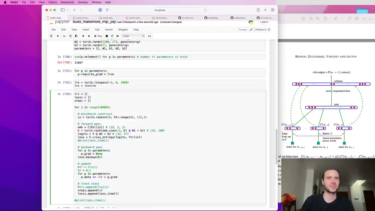 1:07:58
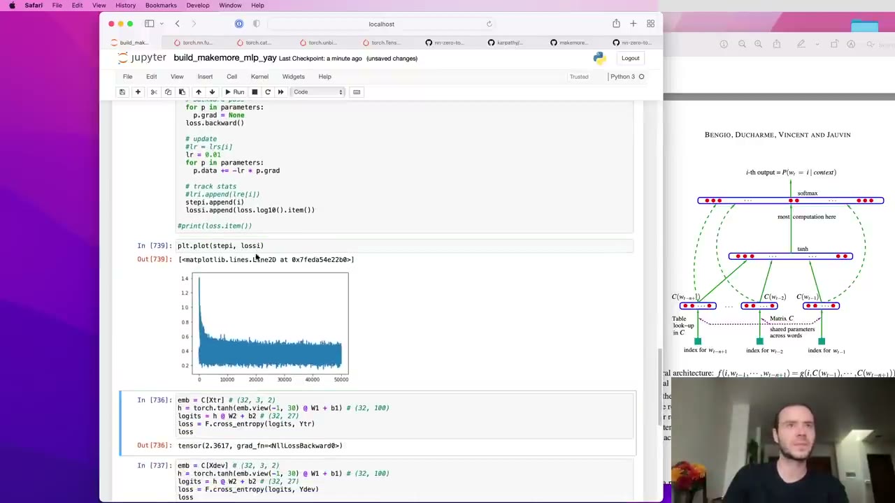 1:10:10
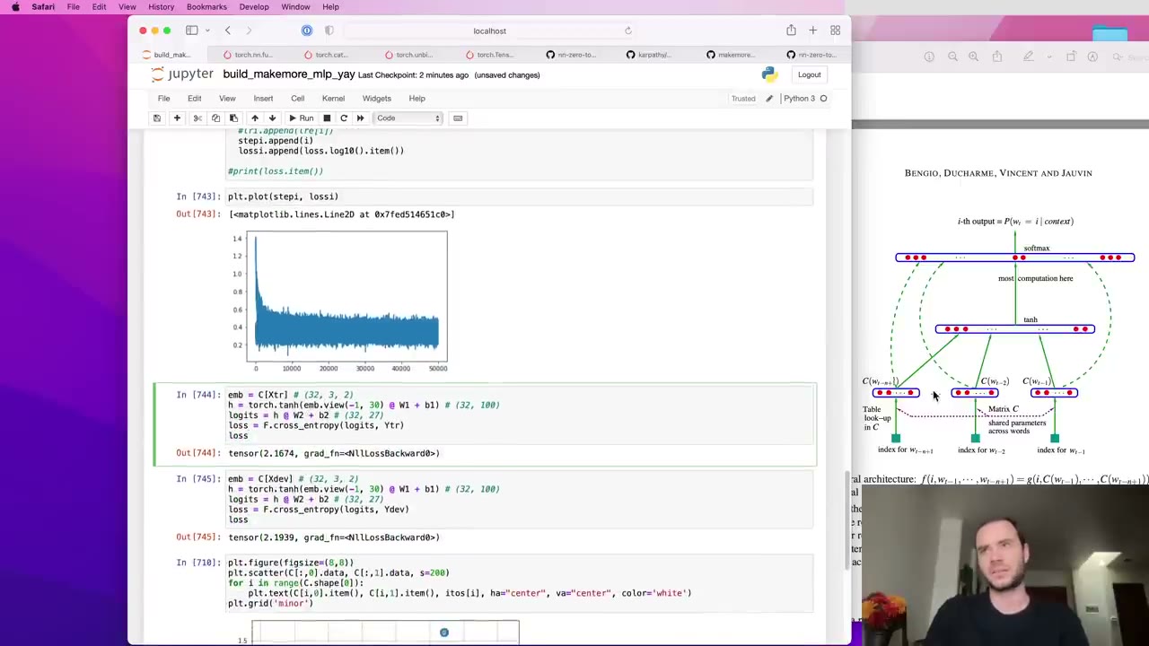 1:11:31
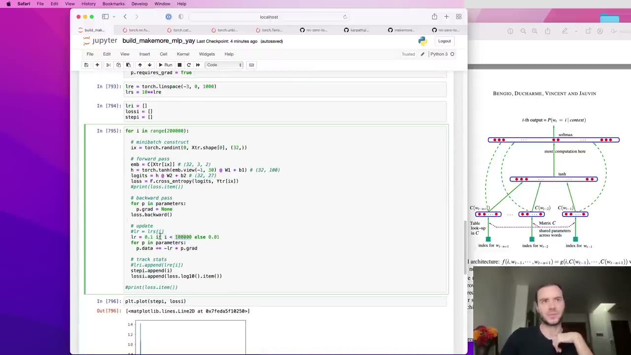 1:11:53
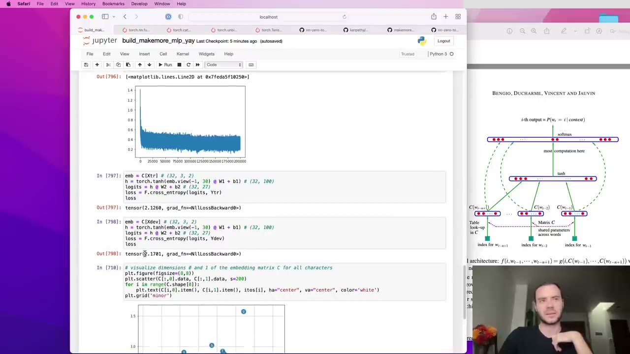 1:12:05
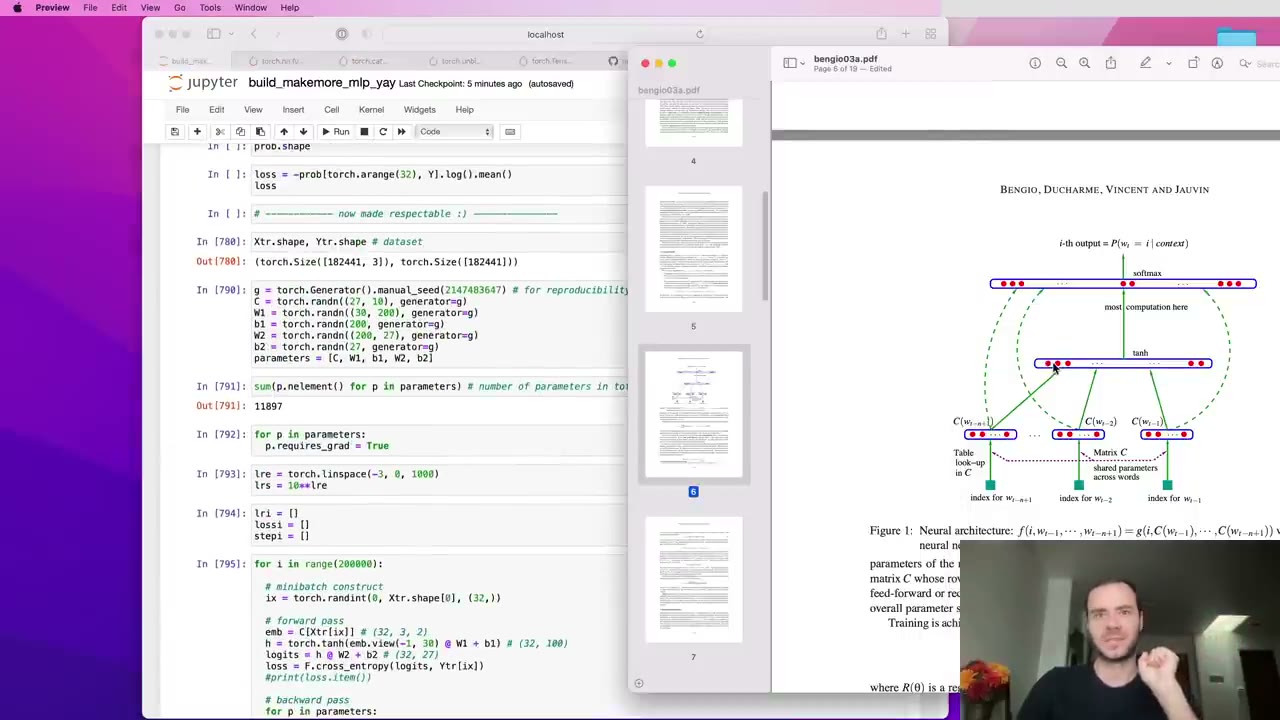 1:12:20
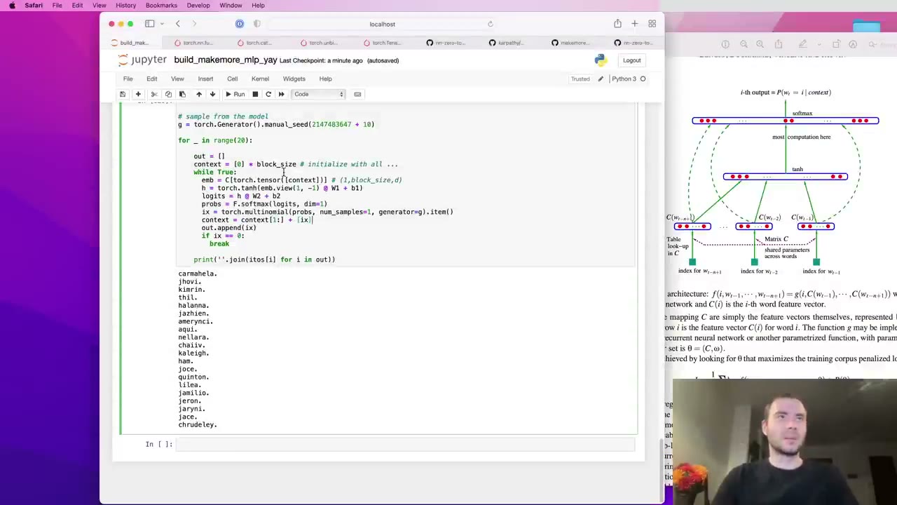 1:13:27
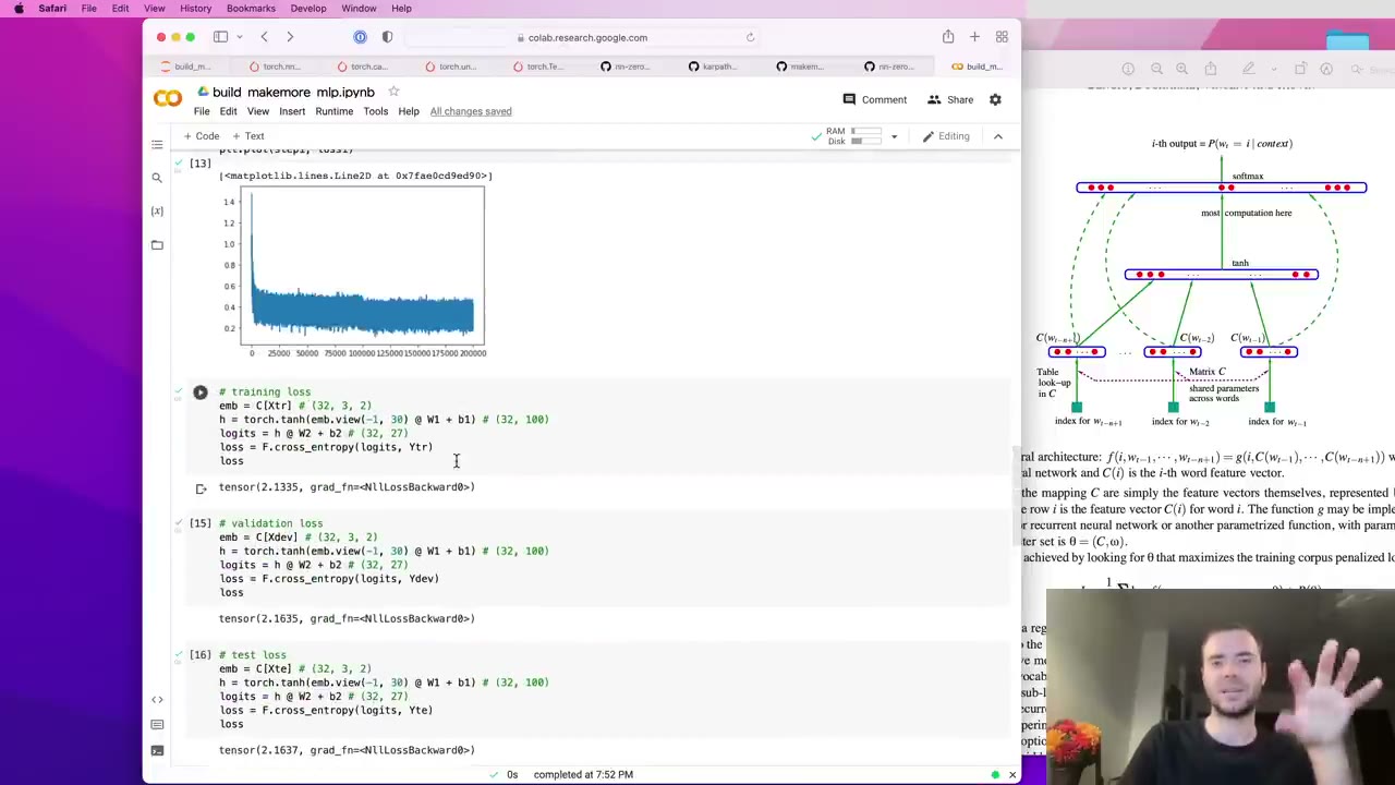 1:15:32
Watch the video (76 min)
Watch the original video on YouTube
Lecture 3 of Andrej Karpathy’s Neural Networks: Zero to Hero picks up the makemore name generator where Lecture 2 left it. The bigram model looked at one previous character, and counting tables cannot simply be extended to longer contexts because the number of possible contexts multiplies by 27 with every extra character. Karpathy’s way out is the neural language model of Bengio et al. (2003): give every character a small learned vector, feed the last few vectors through a hidden layer, and let backpropagation arrange the vectors so that similar characters share what they learn. Most of the 76 minutes is hands-on PyTorch work, and it brings in habits the rest of the series depends on: indexing into an embedding table, reshaping with view, using F.cross_entropy, minibatch training, sweeping the learning rate, and keeping separate train, dev and test splits. The model ends at a validation loss of about 2.17, down from the bigram’s 2.45. Lecture 4 then looks inside this same network at its activations and gradients.
Key takeaways
- Counting tables do not scale with context (1:03). With 27 symbols, two characters of context give 729 rows and three give roughly 20,000, far too many for each row to collect useful counts.
- Embeddings let the model generalize to contexts it has never seen (4:40). If two tokens behave alike, training pulls their vectors together, and what the network learns about one carries over to the other.
- An embedding lookup is the same as a one-hot input times a weight matrix (15:14). Indexing gives an identical result and is much faster, so the one-hot view is dropped.
viewreshapes a tensor without moving any memory (24:32). It only changes how the flat storage is interpreted, which makes it the cheap way to join the three embeddings into one row;torch.catcopies.- Use
F.cross_entropyrather than hand-rolled softmax plus log-likelihood (33:24). It is faster forward and backward, and it guards against overflow by subtracting the largest logit. - Many noisy minibatch steps beat a few exact full-batch steps (43:50). A gradient estimated on 32 examples points roughly the right way, and you can take far more of them.
- Pick the learning rate with a sweep, not a guess (47:29). Spacing candidates exponentially and plotting loss against the exponent shows where training is too slow and where it blows up.
- Read train and dev loss together (1:00:08). Equal losses mean the model is underfitting and can grow; a widening gap means it has started to overfit.
Chapter notes
0:01 – 8:57 From count tables to Bengio’s neural language model
Karpathy recaps the previous notebook: the bigram model, built once from normalized counts and once as a single linear layer, sees only one character before predicting the next, and its samples did not sound much like names. Adding context to a count table is the obvious fix, but the table grows exponentially with the context length (1:03): 27 rows for one character, 729 for two, about 20,000 for three. Spread over a dataset of roughly 32,000 names, most rows would see almost no data.
So the plan changes to a multi-layer perceptron, following Bengio et al. 2003 (1:34). He is clear that it was not the first neural language model, but it was influential and is the paper usually cited for the idea.
Our note: the paper is “A Neural Probabilistic Language Model” (Bengio, Ducharme, Vincent and Jauvin), published in the Journal of Machine Learning Research. The MLP class in the makemore repo cites it in its docstring.
The paper works on words with a 17,000-word vocabulary; makemore keeps characters but borrows the design (2:37). Every token gets a feature vector, 30 numbers in the paper’s example. The vectors start out random and are moved by backpropagation during training, so tokens used in similar ways tend to end up near each other.
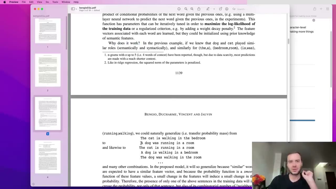
Why that helps is the heart of the lecture’s first half. Karpathy walks through the paper’s example (4:08): the model must complete “A dog was running in a ___” but never saw that exact phrase. If it has seen “The dog was running in a ___”, and has learned that “a” and “the” are often interchangeable, their embeddings sit close together and the knowledge transfers. The same reasoning lets cats stand in for dogs, or walking for running.
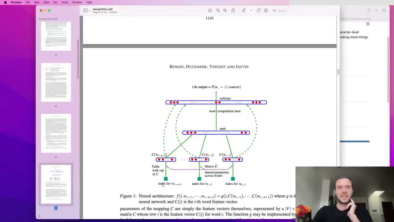
The architecture, read off the paper’s figure (5:42):
- Inputs: the integer indices of the previous three tokens.
- Lookup table C: one row per vocabulary item, shared by all three positions (6:19). Three 30-dimensional vectors make a 90-number input.
- Hidden layer: fully connected, followed by tanh. Its width is a hyperparameter, a design choice left to the builder (6:50).
- Output layer: one logit per vocabulary item, which makes it the expensive layer when the vocabulary is 17,000 words (7:54).
- Softmax and loss: logits become a probability distribution, and training maximizes the probability of the true next token. The trainable parameters are both layers’ weights and biases plus C (8:25).
He tells viewers to ignore the dashed arrows in the figure, a variant he doesn’t cover.
8:57 – 12:06 A dataset built from a rolling window
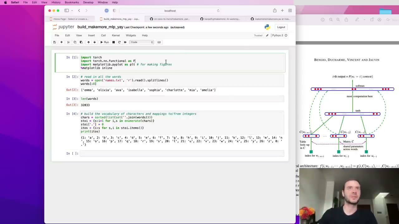
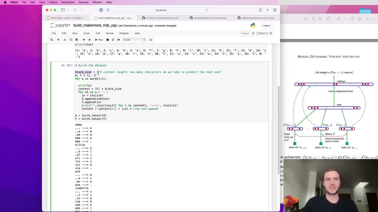
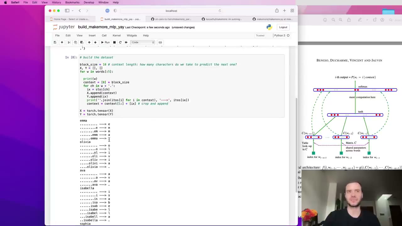
A fresh notebook loads the names and the character-to-integer mappings from last time (8:57). The new piece is the dataset. block_size sets how many characters of context support each prediction (9:28); with 3, the name “emma” turns into five examples, starting from a context of three padding dots that should predict “e” (10:32). The context then slides along one character at a time: drop the oldest, append the newest.
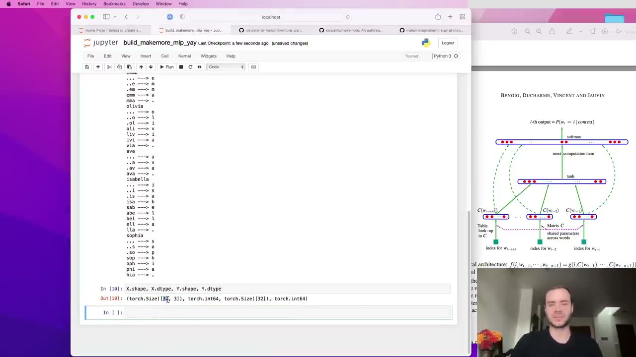
Changing block_size to 4, 5 or 10 changes only the window length, with the padding dots filling in at the start (11:04). While developing he uses only the first five names, which yields 32 examples: an X of shape 32×3 and a Y of 32 labels (11:36).
12:06 – 18:20 The embedding table and PyTorch indexing
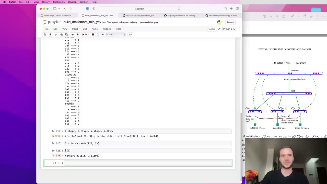
With only 27 characters, Karpathy starts with a tiny embedding: C is a random 27×2 matrix, so every character becomes a point in a plane (12:38).
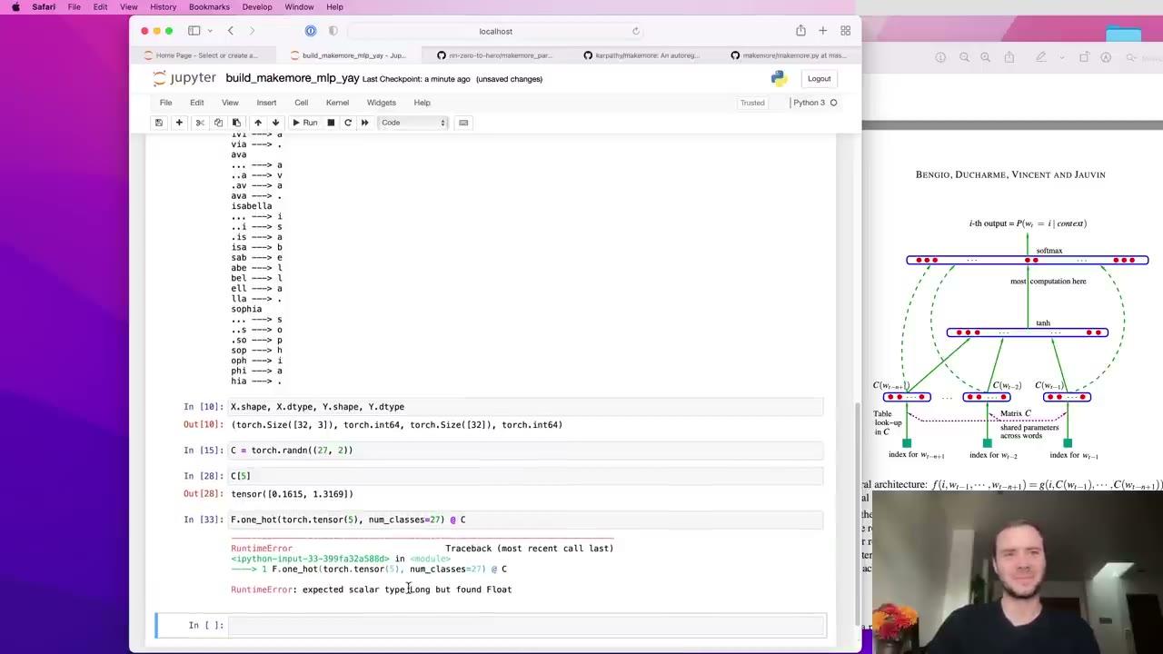
He then shows that two descriptions of the lookup are the same operation (13:10). Indexing C[5] returns row 5. Alternatively, one-hot encode 5 into a 27-long vector and matrix-multiply it by C; the zeros mask out every row except row 5. Getting there produces two deliberate errors: F.one_hot needs a tensor rather than a Python int, and the one-hot result is a 64-bit integer type that must be cast to float before it can multiply a float matrix (14:43). The takeaway (15:14) is that the embedding can be read as a first linear layer with no nonlinearity whose weight matrix is C. Indexing is faster, so that is what the code uses.
Embedding a whole batch at once relies on PyTorch’s flexible indexing (16:18). You can index with a list, with an integer tensor, with repeated indices, and with a two-dimensional integer tensor. C[X] therefore returns shape 32×3×2: an embedding for each of the 32×3 integers. He spot-checks one entry against C indexed directly (17:49).
18:20 – 29:15 The hidden layer: joining embeddings with view
The hidden layer takes 3 × 2 = 6 inputs and starts with 100 neurons (18:20). The obstacle: emb is 32×3×2, and a 6×100 weight matrix needs a 32×6 input (19:22).
Karpathy uses this to show that a large library usually offers several routes, some better than others (19:53). The first is torch.cat on the three slices emb[:, 0, :], emb[:, 1, :] and emb[:, 2, :] along dimension 1, which works but hard-codes a block size of 3 (21:57). The second, torch.unbind(emb, 1), produces the same list of slices for any block size (22:27).
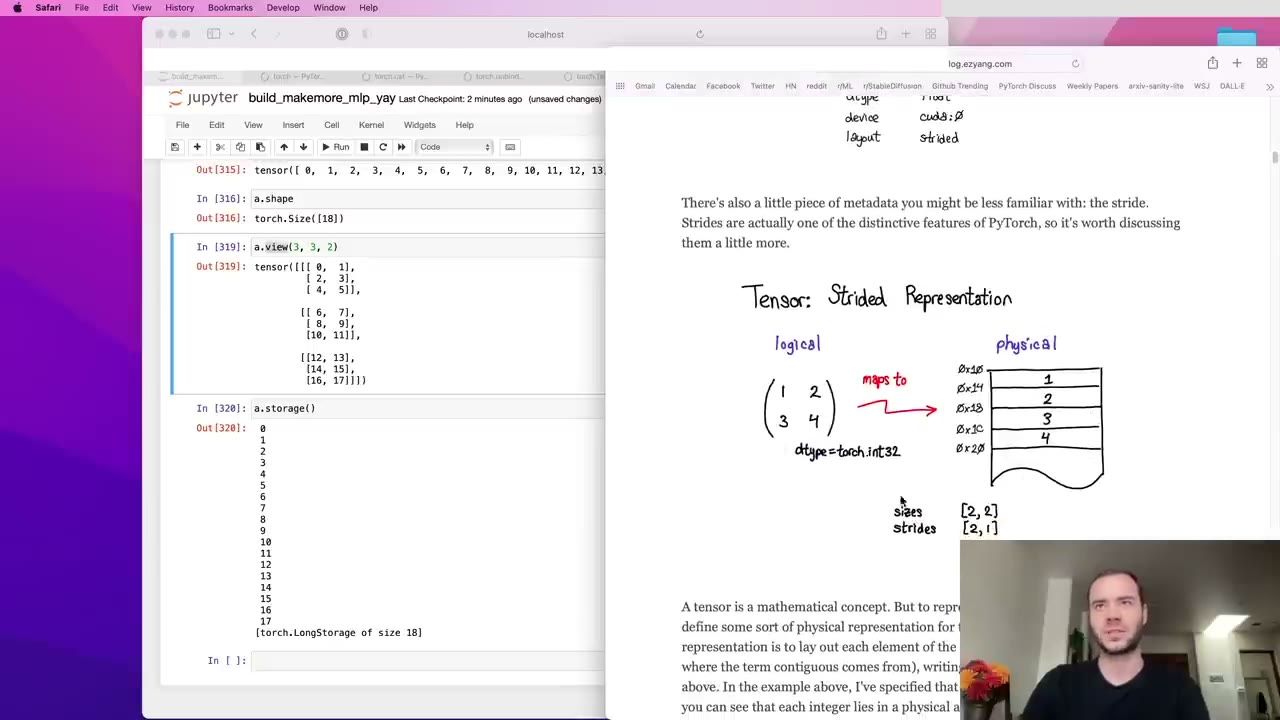
The better answer is view (23:30). A tensor of 18 numbers can be viewed as 2×9, 9×2 or 3×3×2 as long as the element count matches. The reason this is nearly free (24:32): every tensor sits on a one-dimensional storage, and its shape, strides and storage offset only say how to read that storage. view changes those attributes and copies nothing. Karpathy points to Edward Z. Yang’s blog post on PyTorch internals for the details (25:05).
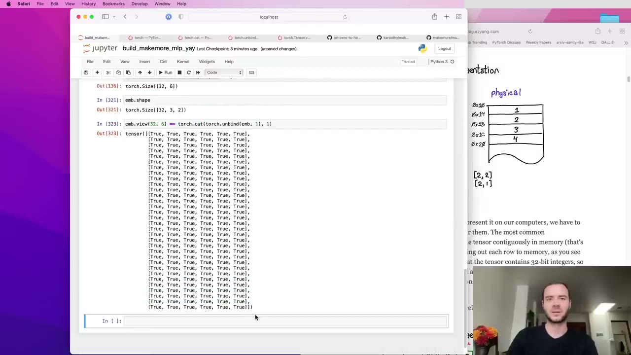
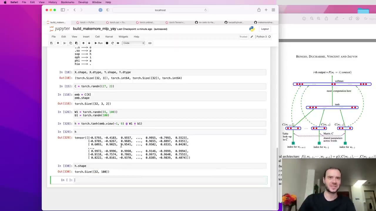
Viewing emb as 32×6 happens to lay each example’s three embeddings side by side, which is exactly the concatenation, and an element-wise comparison confirms it (26:07). Writing -1 instead of 32 lets PyTorch infer that dimension (27:09). In contrast, torch.cat must allocate new storage, because no change of view can join separate tensors (27:39). Adding tanh gives h, 32×100 activations between -1 and 1.
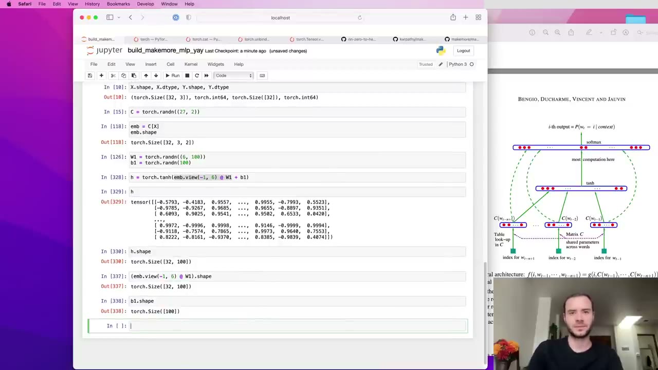
The last check is the bias addition (28:10). A 32×100 matrix plus a 100-vector broadcasts by aligning on the right, treating the bias as a 1×100 row and copying it down all 32 rows. That is the intended behavior, and Karpathy recommends checking broadcasts like this every time.
Our note: view only works when the requested shape is compatible with the tensor’s current strides. A freshly created tensor such as emb is fine; after operations like a transpose you may need .contiguous() first or reshape, which copies only when it has to.
29:15 – 37:33 Output layer, the loss, and why F.cross_entropy wins
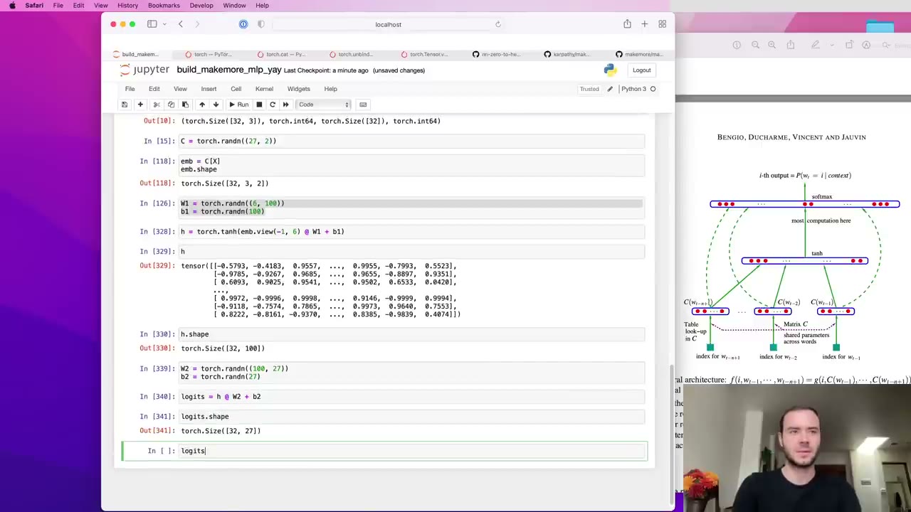
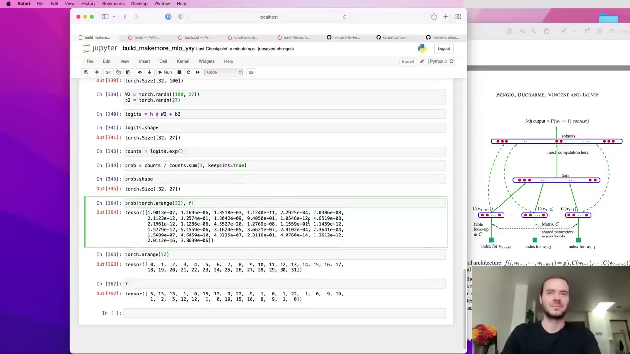
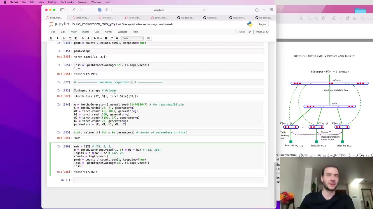
W2 is 100×27 and b2 has 27 entries, one per possible next character, so logits = h @ W2 + b2 is 32×27 (29:15). From there the steps match Lecture 2: exponentiate to get “fake counts”, divide by the row sums to get probabilities (29:47), then use torch.arange(32) with Y to pick out the probability each row gives to the correct character (30:50). Untrained, some are near 0.2 and some are tiny. The mean negative log probability, the negative log-likelihood, comes out at about 17.3 (31:52).
Our note: 17 is far above the roughly 3.3 (that is, ln 27) you would expect from a model guessing uniformly over 27 characters. The weights here come straight from torch.randn, which makes the initial logits large and confidently wrong. Lecture 4 starts by fixing exactly this.
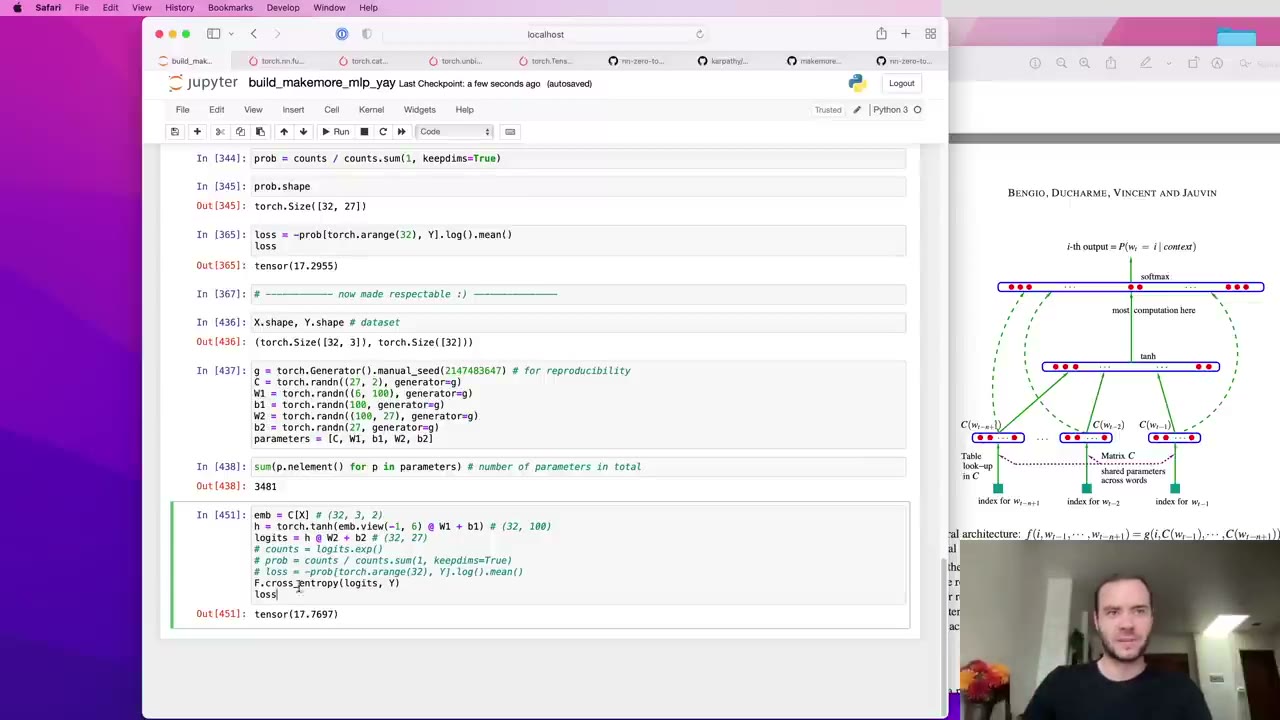
Karpathy cleans the notebook: a seeded torch.Generator makes runs reproducible, and all tensors go into one parameters list, about 3,400 numbers at this size (32:23). The three hand-written loss lines are then replaced by one call to F.cross_entropy(logits, Y), which gives the same value (32:53).
His reasons to always prefer the built-in (33:24):
| Reason | What happens |
|---|---|
| Efficient forward pass | No intermediate tensors; the operations can run as one fused kernel |
| Efficient backward pass | The combined derivative is derived analytically and is much simpler, like micrograd’s tanh backward of 1 − t² (34:28) |
| Numerical safety | Very large logits are handled without overflow (34:59) |
The demonstration of the third point: very negative logits are harmless, because exp just returns numbers near zero. A logit of +100, though, makes exp overflow to inf and the probabilities become NaN (36:00). Because softmax normalizes, adding or subtracting a constant from all logits leaves the probabilities unchanged (36:32), so PyTorch subtracts the maximum logit first. The largest value becomes 0, everything else goes negative, and nothing can overflow.
Our note: F.cross_entropy expects raw logits and applies softmax itself. Passing it probabilities you have already normalized is a common bug that still runs but trains badly.
37:33 – 45:24 Training: one batch first, then minibatches
The loop has three steps (38:05): set each p.grad to None (PyTorch’s equivalent of zeroing), call loss.backward(), and nudge each parameter’s data by minus the learning rate times its gradient. It needs requires_grad = True on every parameter first (38:39).
On the 32 development examples the loss falls from 17 to very low values (39:10). That is easy: 3,400 parameters against 32 examples is overfitting a single batch. It can’t reach zero, and Karpathy shows why (40:11). The context of three dots is followed by a different first letter in each of the five names (e, o, a, i and s), so no single prediction can be right for all of them. Where an input has exactly one answer, the network does memorize it.
Building from all names gives 228,146 examples (41:13), and each full forward and backward pass becomes slow. The standard fix is minibatches (42:15): torch.randint draws 32 random row indices, and both X and Y are indexed with them. Iterations become almost instant (43:50).
The trade-off is a noisier gradient that is no longer the exact direction, but Karpathy argues that an approximate gradient with many more steps works better than an exact one with few. Since one minibatch’s loss is itself noisy, he evaluates on all of X and Y to judge progress: about 2.7, then 2.6, then 2.53 as training continues (44:53).
45:24 – 53:16 Finding a learning rate, then decaying it
The 0.1 he had been using was a guess (45:24). His method has two stages. First, bracket by hand with short runs: 0.0001 barely moves the loss, 0.001 lowers it slowly, 1 decreases it but unsteadily, and 10 fails outright, so the useful range is roughly 0.001 to 1 (46:26). Second, sweep that range systematically (46:57). Rather than spacing 1,000 learning rates linearly, he spaces their exponents linearly from -3 to 0 and raises 10 to those powers, so the candidates are spread evenly on a log scale (47:29).
One run of 1,000 steps then uses candidate i at step i, from 0.001 up to 1, while recording the rate and the loss (48:30). Plotted against the exponent (50:07), the curve is flat on the left, dips into a valley, and turns unstable on the right. The valley is near -1, so 0.1 was a sensible choice after all.
Our note: because the rate rises as training goes on, each point mixes the effect of the rate with how far training has already progressed. That is fine for finding a rough range, which is all Karpathy uses it for.
With 0.1 confirmed, he runs 10,000 steps at a time (51:40): about 2.48, then 2.46. That already beats the bigram’s 2.45 (52:12). When progress flattens, he cuts the rate tenfold for the last stretch, a learning-rate decay, and reaches about 2.3 (52:46). He calls the procedure janky but representative: find a rate, train with it, decay at the end.
53:16 – 58:31 Train, dev and test splits
Karpathy then admits that “better than the bigram” was not yet a fair claim (53:16). As a network gains parameters it can overfit, driving training loss toward zero by memorizing the data. Its samples then copy training names, and its loss on held-out names is high.
The standard defense is three splits (54:19), roughly 80/10/10:
- Training split: fits the parameters with gradient descent.
- Dev (validation) split: compares hyperparameters such as hidden-layer size, embedding size and regularization strength (55:21).
- Test split: measures final performance, and only a few times, because each look that influences your choices is a little training on the test set (55:51).
In code (56:24), dataset construction becomes a build_dataset(words) function. The names are shuffled and cut at 80% and 90%: of 32,033 names, 25,626 go to training, 3,203 to dev and 3,204 to test. The splits are made at the level of names, then each split is turned into examples.
58:31 – 1:04:23 Underfitting, and a wider hidden layer
Training now uses only Xtr and Ytr (58:31). After fixing an accidentally decayed learning rate, the dev loss is about 2.3 and the training loss is about the same (1:00:08). Equal losses mean underfitting: the network is too small to memorize anything, so a bigger one should help.
The hidden layer goes from 100 to 300 neurons, 10,281 parameters (1:00:38). He starts logging step and loss to plot training (1:01:41); the curve is thick with minibatch noise, and he mentions a larger batch size as one way to steady the gradient (1:02:42). Progress is slow: 2.5, then 2.32 after halving the rate, then 2.23 (1:04:23). Tripling the hidden layer has not bought much, which suggests the bottleneck is elsewhere.
1:04:23 – 1:07:01 The 2D embeddings as a picture
His suspicion is the two-dimensional embeddings: 27 characters crammed into a plane may be the limit (1:04:23). Before enlarging them he takes the last chance to plot them, using the two columns of C as x and y and labeling each point with its character (1:05:28).
The picture has structure (1:05:59). The vowels a, e, i, o and u cluster together, so the network treats them as roughly interchangeable. The letter q sits far away with an embedding of its own, as does the special dot token, and most consonants bunch together. The table started random; training organized it.
1:07:01 – 1:13:12 Bigger embeddings and the 2.17 challenge
The new settings are 10-dimensional embeddings, 30 inputs to the hidden layer and 200 hidden neurons, 11,897 parameters (1:07:01). He fixes the hard-coded 6 that had to become 30 and moves initialization into its own cell so reruns don’t wipe the log (1:08:02). He also logs the base-10 log of the loss, which flattens the hockey-stick shape of the plot (1:08:32).
Results: training 2.3 and dev about 2.38, then after a decay 2.17 and 2.2 (1:10:07). The gap is starting to open, a first hint of overfitting, and the improvement confirms the embedding size was holding the model back (1:11:08). Karpathy is candid that this hand-tuning is haphazard; in production every setting would become a hyperparameter explored by many experiments, judged on dev, with one final test evaluation to report (1:10:38).
A cleaned-up run of 200,000 steps, at 0.1 for the first half and 0.01 for the second, reaches a best validation loss of 2.17 (1:11:38). He leaves beating it as an exercise and lists the knobs (1:12:10): hidden size, embedding size, context length, training length, learning rate and its decay schedule, and batch size. He also recommends reading the Bengio paper, which he says viewers can now largely follow and which contains more ideas to try.
1:13:12 – end Sampling names, plus a Colab
Generation starts from a context of three dots and loops until the model produces the end token (1:13:12). Each step embeds the current context as a batch of one, runs it through the hidden layer to get logits, and turns them into probabilities with F.softmax, which, like cross-entropy, protects against overflow (1:13:43). torch.multinomial draws the next index, and the window slides forward. The samples sound much more like names than the bigram’s, though still with room to improve (1:14:13).
To spare viewers a local install of Jupyter and PyTorch, Karpathy shares a Google Colab version of the notebook, slightly shortened, that trains, plots and samples in the browser (1:14:44). The link is in the video description.
Code you’ll write
These are short excerpts in the spirit of the lecture notebook. The complete version is makemore_part2_mlp.ipynb in nn-zero-to-hero, and the makemore repo has a packaged MLP model in makemore.py. Both are MIT-licensed. They assume words, stoi, itos, torch and torch.nn.functional as F from the notebook’s setup.
1. Turning names into (context, next character) examples. A rolling window of block_size integers is the input and the following character is the label; the function form is applied separately to each split (9:28, split version at 56:24).
import random
block_size = 3  # context length

def build_dataset(words):
    X, Y = [], []
    for w in words:
        context = [0] * block_size
        for ch in w + '.':
            ix = stoi[ch]
            X.append(context)
            Y.append(ix)
            context = context[1:] + [ix]  # crop and append
    return torch.tensor(X), torch.tensor(Y)

random.seed(42)
random.shuffle(words)
n1, n2 = int(0.8 * len(words)), int(0.9 * len(words))
Xtr, Ytr = build_dataset(words[:n1])
Xdev, Ydev = build_dataset(words[n1:n2])
Xte, Yte = build_dataset(words[n2:])
2. Parameters for the final configuration. A seeded generator, 10-dimensional embeddings and a 200-unit hidden layer, all collected into one list (32:23, resized at 1:07:01).
g = torch.Generator().manual_seed(2147483647)
C  = torch.randn((27, 10), generator=g)
W1 = torch.randn((30, 200), generator=g)
b1 = torch.randn(200, generator=g)
W2 = torch.randn((200, 27), generator=g)
b2 = torch.randn(27, generator=g)
parameters = [C, W1, b1, W2, b2]
for p in parameters:
    p.requires_grad = True
3. The forward pass. Index the embedding table, flatten the context with view, apply the tanh layer and the output layer, and score with cross-entropy (26:38, cross-entropy at 32:53).
emb = C[X]                                   # (N, 3, 10)
h = torch.tanh(emb.view(-1, 30) @ W1 + b1)   # (N, 200)
logits = h @ W2 + b2                         # (N, 27)
loss = F.cross_entropy(logits, Y)
4. Minibatch training with a step-decayed learning rate. Each step draws 32 random examples, zeroes the gradients, backpropagates and updates (42:15, final schedule at 1:11:38).
for i in range(200000):
    ix = torch.randint(0, Xtr.shape[0], (32,))   # minibatch
    emb = C[Xtr[ix]]
    h = torch.tanh(emb.view(-1, 30) @ W1 + b1)
    logits = h @ W2 + b2
    loss = F.cross_entropy(logits, Ytr[ix])
    for p in parameters:
        p.grad = None
    loss.backward()
    lr = 0.1 if i < 100000 else 0.01
    for p in parameters:
        p.data += -lr * p.grad
5. The learning-rate sweep. Candidates spaced evenly in the exponent; inside the loop, step i uses lrs[i] and you record lre[i] and the loss, then plot one against the other (47:29).
lre = torch.linspace(-3, 0, 1000)   # exponents from -3 to 0
lrs = 10**lre                       # learning rates from 0.001 to 1
# in the training loop, for i in range(1000):
#     lr = lrs[i]; ...; lri.append(lre[i]); lossi.append(loss.item())
plt.plot(lri, lossi)
6. Sampling new names. Start from all dots, predict, draw, slide the window, stop at the end token (1:13:12).
g = torch.Generator().manual_seed(2147483647 + 10)
for _ in range(20):
    out, context = [], [0] * block_size
    while True:
        emb = C[torch.tensor([context])]          # (1, block_size, 10)
        h = torch.tanh(emb.view(1, -1) @ W1 + b1)
        logits = h @ W2 + b2
        probs = F.softmax(logits, dim=1)
        ix = torch.multinomial(probs, num_samples=1, generator=g).item()
        context = context[1:] + [ix]
        out.append(ix)
        if ix == 0:
            break
    print(''.join(itos[i] for i in out))
Skip list
- 0:01 – 1:34 Recap of the bigram notebook. Skip if you just finished Lecture 2; the scaling argument is restated in the takeaways above.
- 13:40 – 15:14 The one-hot route to embeddings, including two deliberate type errors. Worth it once for the “embedding is a linear layer” insight; skip on a rewatch.
- 19:53 – 23:30
torch.catandtorch.unbind. Both are discarded in favor ofview; watch only if you want to see why. - 1:01:41 – 1:04:23 Repeated reruns of the 300-neuron model as the loss creeps down. The conclusion, that the embeddings are the bottleneck, comes at 1:04:23.
- 1:14:44 – end The Google Colab announcement.
Glossary
- Character-level language model — a model that predicts text one character at a time from the characters before it.
- Context length (
block_size) — how many previous tokens the model sees when predicting the next one; 3 in most of this lecture. - Embedding — a short learned vector that stands for a token; tokens used in similar ways drift toward similar vectors during training.
- Embedding table (C) — the matrix whose rows are the embeddings, one per vocabulary item, shared across all context positions.
- Multi-layer perceptron (MLP) — a network of fully connected layers with nonlinearities between them; here, one tanh hidden layer and an output layer.
- Hyperparameter — a setting chosen by the designer rather than learned, such as hidden-layer width, embedding size or learning rate.
- Logits — the raw, unnormalized scores from the last layer; softmax turns them into probabilities.
- Cross-entropy loss — the average negative log probability the model gives to the correct next token; for this setup it equals the negative log-likelihood Karpathy writes by hand.
view— a PyTorch method that reinterprets a tensor’s existing storage with a new shape, without copying.- Broadcasting — PyTorch’s rule for combining tensors of different shapes by aligning dimensions from the right and stretching size-1 dimensions.
- Minibatch — a small random subset of training examples used to estimate the gradient for one update.
- Learning-rate decay — lowering the learning rate late in training so the parameters settle instead of bouncing.
- Overfitting / underfitting — fitting the training data so closely that held-out loss suffers, versus a model too small to fit even the training data; compare train and dev loss to tell them apart.
- Train / dev / test split — separate portions of the data for fitting parameters, choosing hyperparameters, and a final, rarely used performance check.
FAQ
What model does Karpathy build in makemore Part 2?
A character-level version of the multi-layer perceptron language model from Bengio et al. (2003). Each of the previous three characters is looked up in a learned embedding table C, the vectors are joined into one input, passed through a tanh hidden layer, and an output layer produces 27 logits, one per possible next character. Embeddings, weights and biases are all trained together with backpropagation.
Why does Karpathy use F.cross_entropy instead of writing the loss by hand?
He gives three reasons. PyTorch can run the whole calculation as a fused kernel without creating intermediate tensors; the backward pass is simpler and cheaper because the derivative is worked out analytically; and it is numerically safe, because it subtracts the largest logit before exponentiating, so very large logits do not overflow to inf and produce NaN.
How does Karpathy choose the learning rate in the MLP lecture?
He first brackets the range by hand: very small rates barely move the loss and 10 makes training fail, which points to a range of about 0.001 to 1. He then runs 1,000 steps while raising the learning rate exponentially from 0.001 to 1, records the loss at each step, and plots loss against the exponent. The valley sits near an exponent of -1, so he trains at 0.1 and later decays to 0.01.
What loss does the MLP reach compared with the bigram model?
The bigram model from the previous lecture reached about 2.45. The first small MLP passes it within minutes of training and gets to about 2.3. After widening the embeddings to 10 dimensions and training 200,000 steps with one learning-rate decay, Karpathy's best validation loss is 2.17, which he leaves as a number for viewers to beat.
Why split the data into train, dev and test sets?
A large enough network can memorize its training set, so a low training loss alone does not prove the model is good. The training split (about 80%) fits the parameters, the dev or validation split (about 10%) is used to compare hyperparameters such as layer sizes, and the test split (about 10%) is checked only a few times at the end, so that you do not end up tuning to it as well.
Studying another course? Paste its YouTube or Bilibili link on the home page to request a handout — or make your own with the desktop app (coming soon).