Karpathy's Zero to Hero, Lecture 1: Building micrograd — notes, code and timestamps
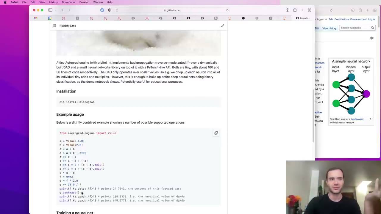 2:59
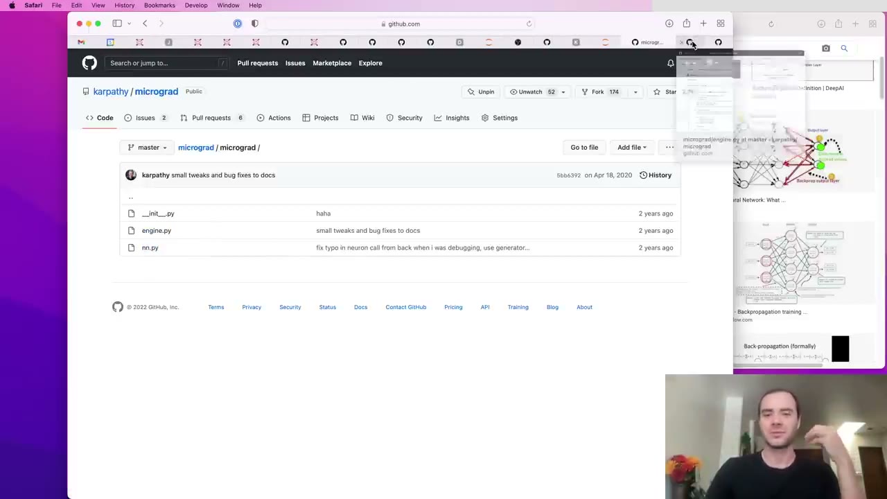 7:18
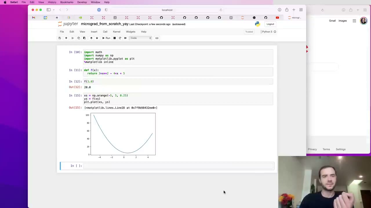 9:45
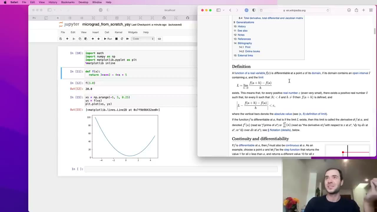 10:48
 12:59
 17:40
 22:57
 24:41
 25:33
 29:00
 31:54
 37:02
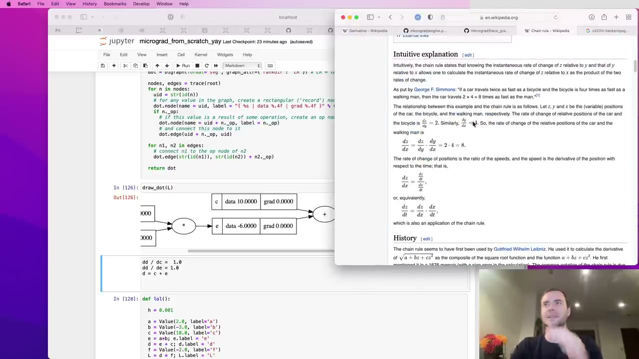 42:58
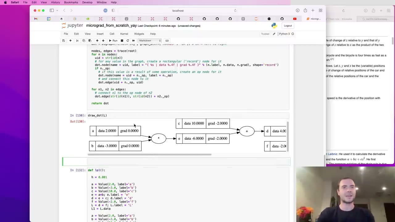 47:23
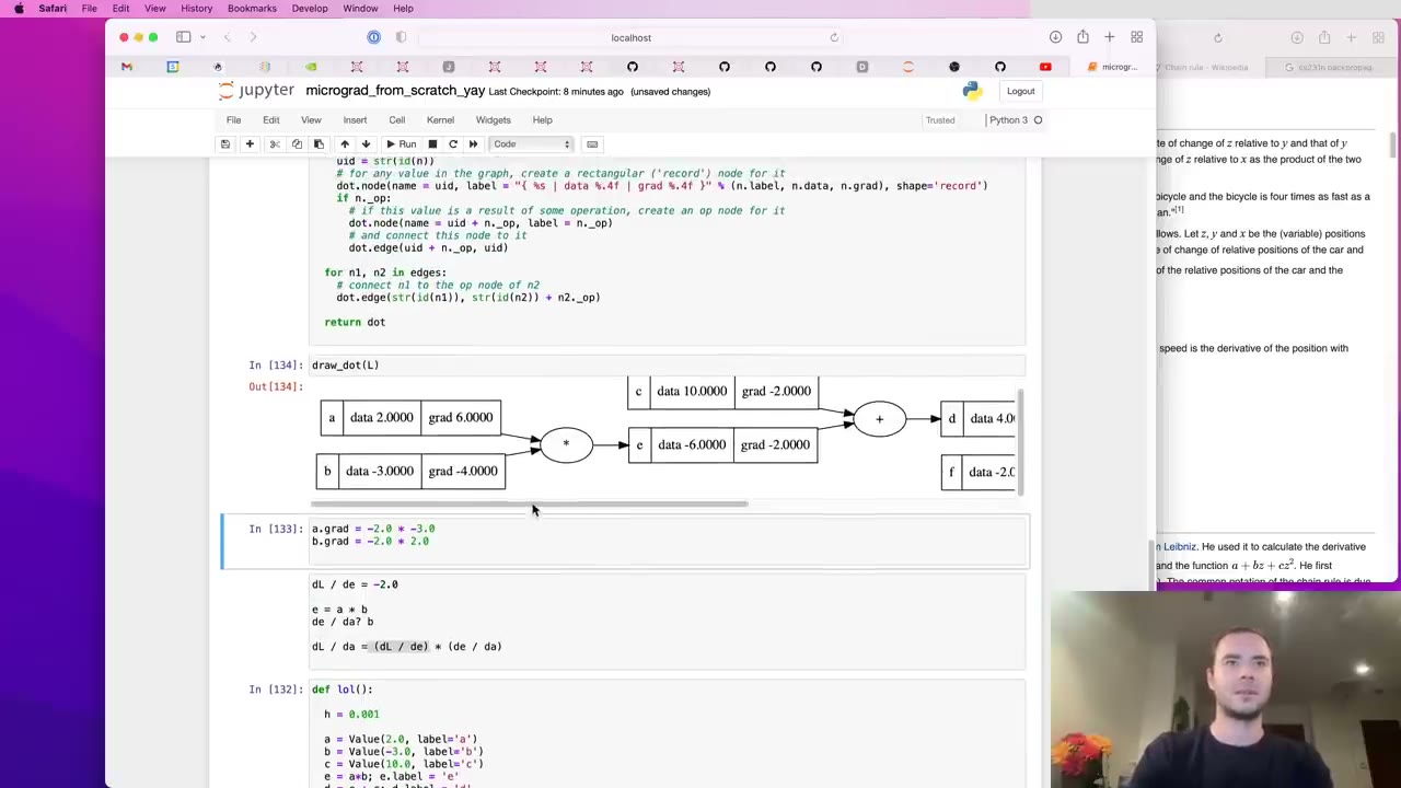 49:32
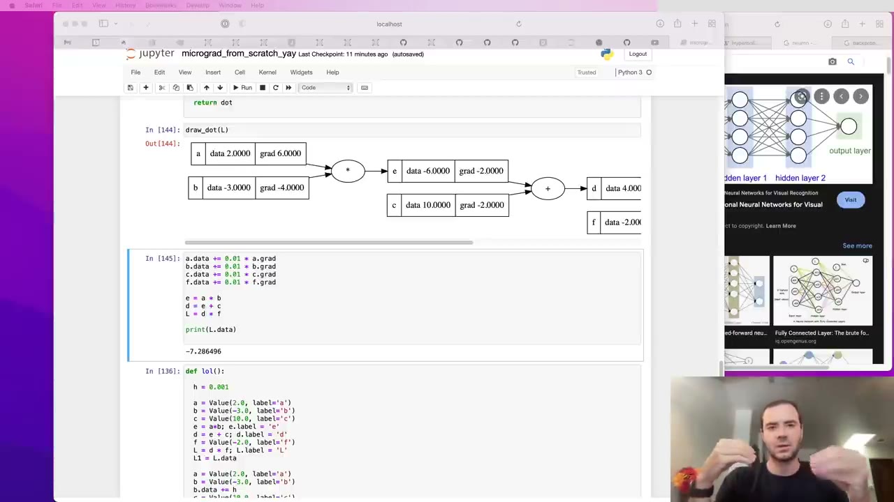 52:55
 53:27
 54:36
 56:45
 1:00:00
 1:01:22
 1:04:24
 1:08:49
 1:14:21
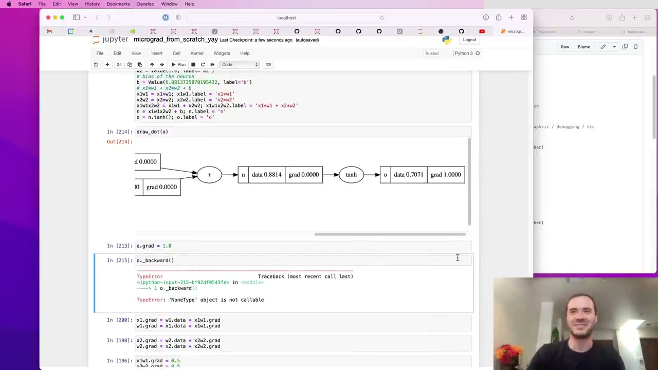 1:15:20
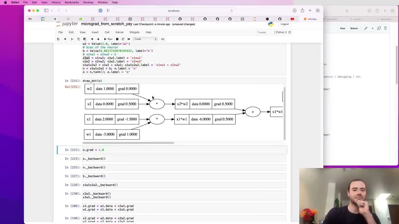 1:17:19
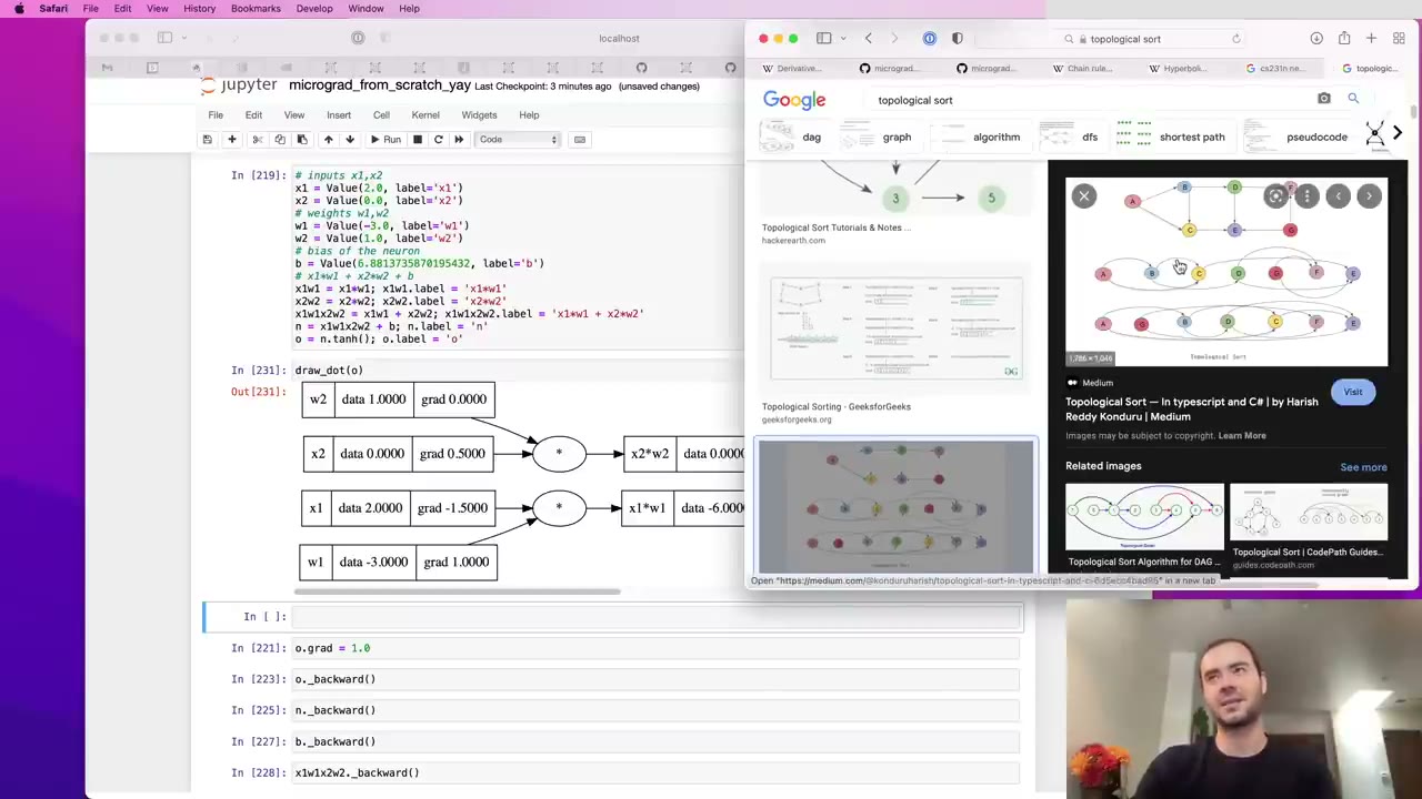 1:18:26
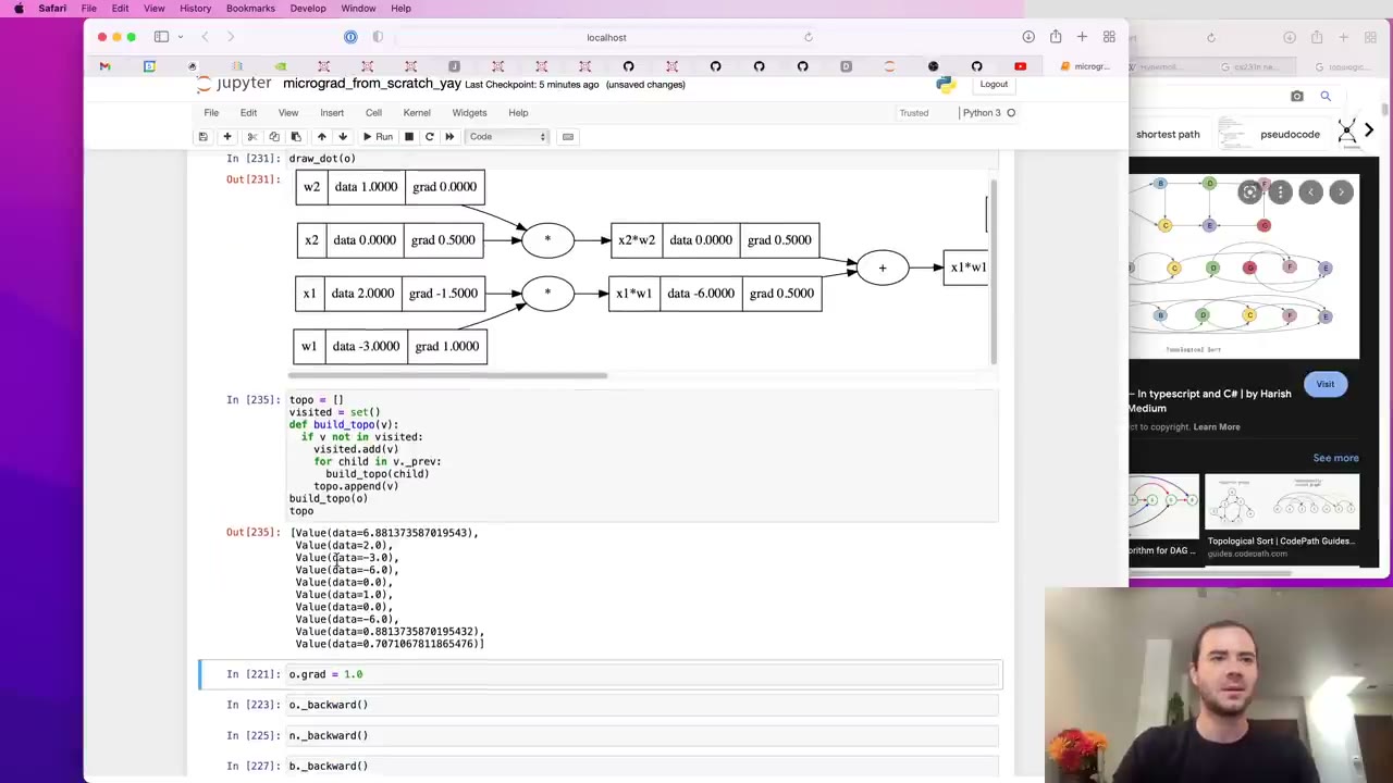 1:19:52
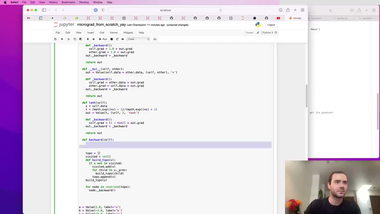 1:21:35
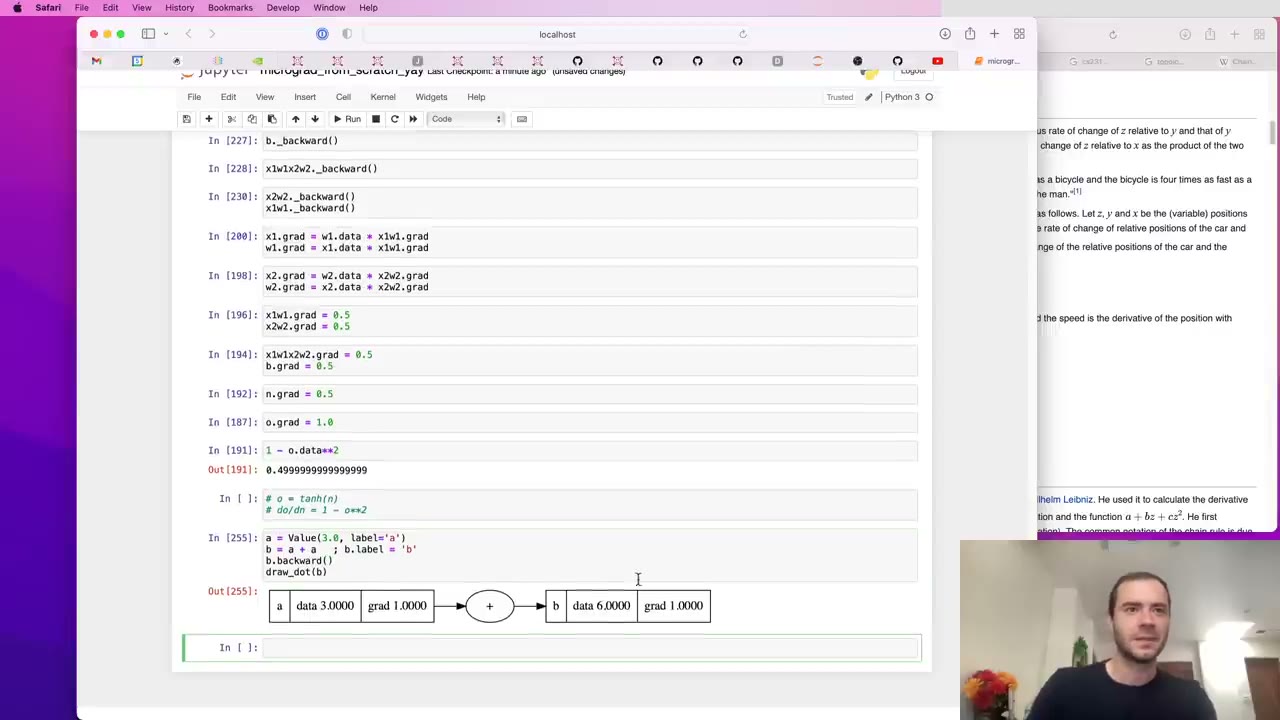 1:22:54
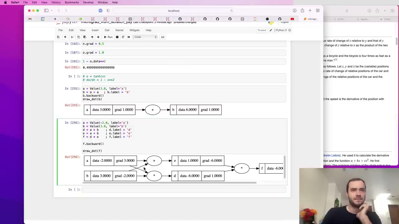 1:24:25
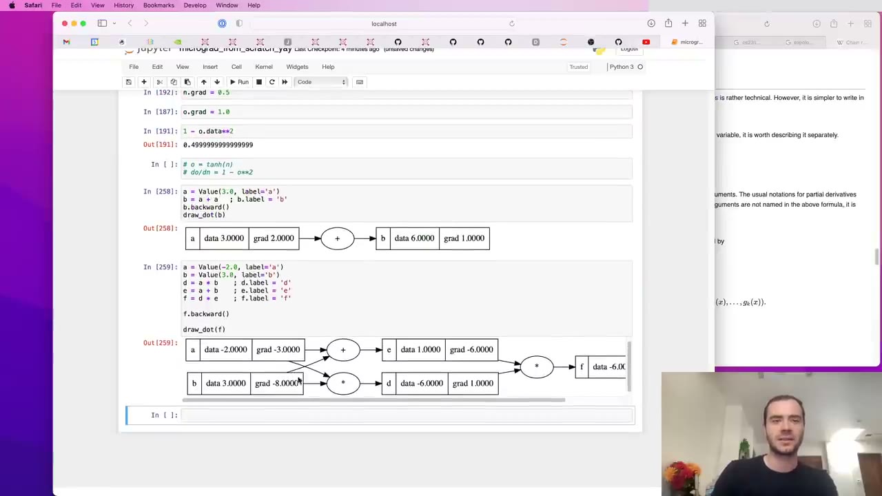 1:26:18
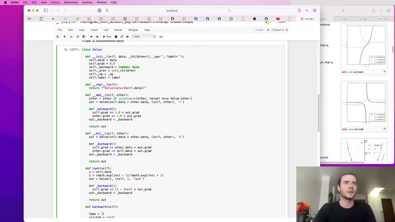 1:28:32
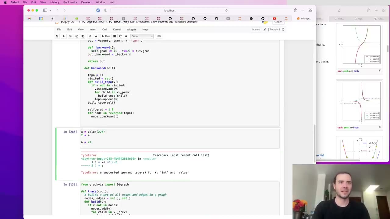 1:29:31
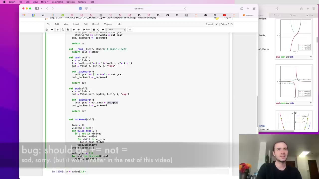 1:31:32
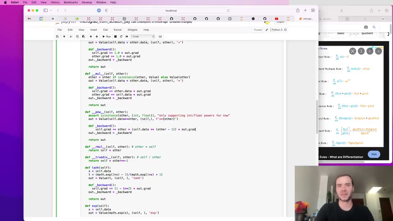 1:35:35
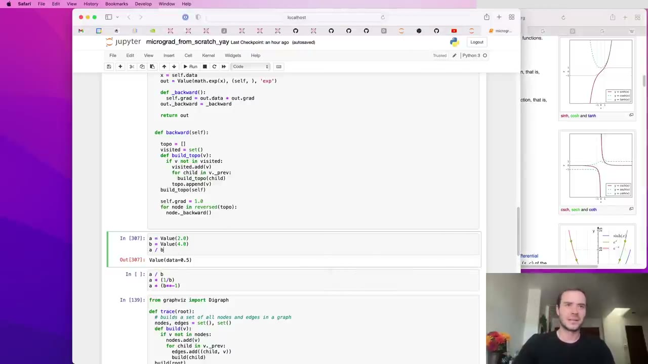 1:35:55
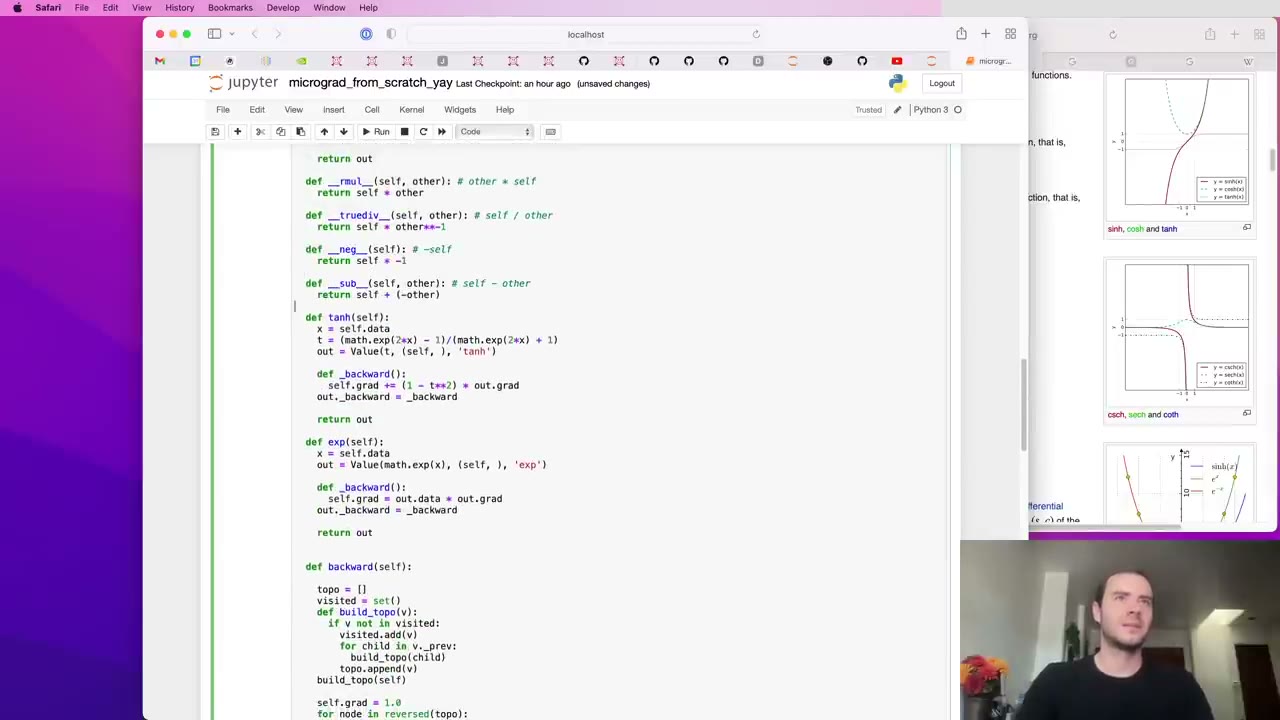 1:36:03
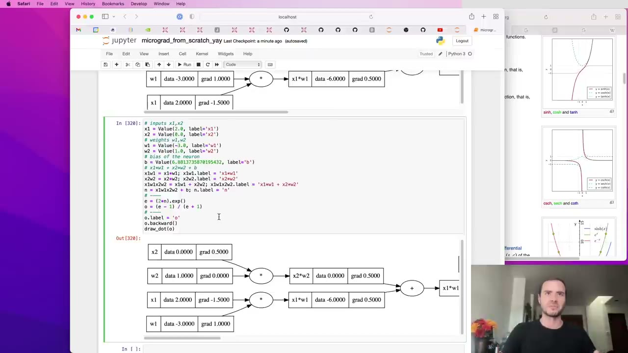 1:39:03
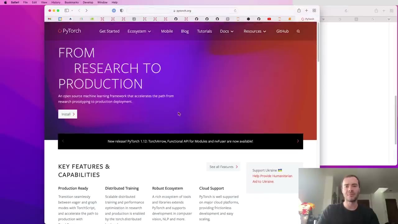 1:39:40
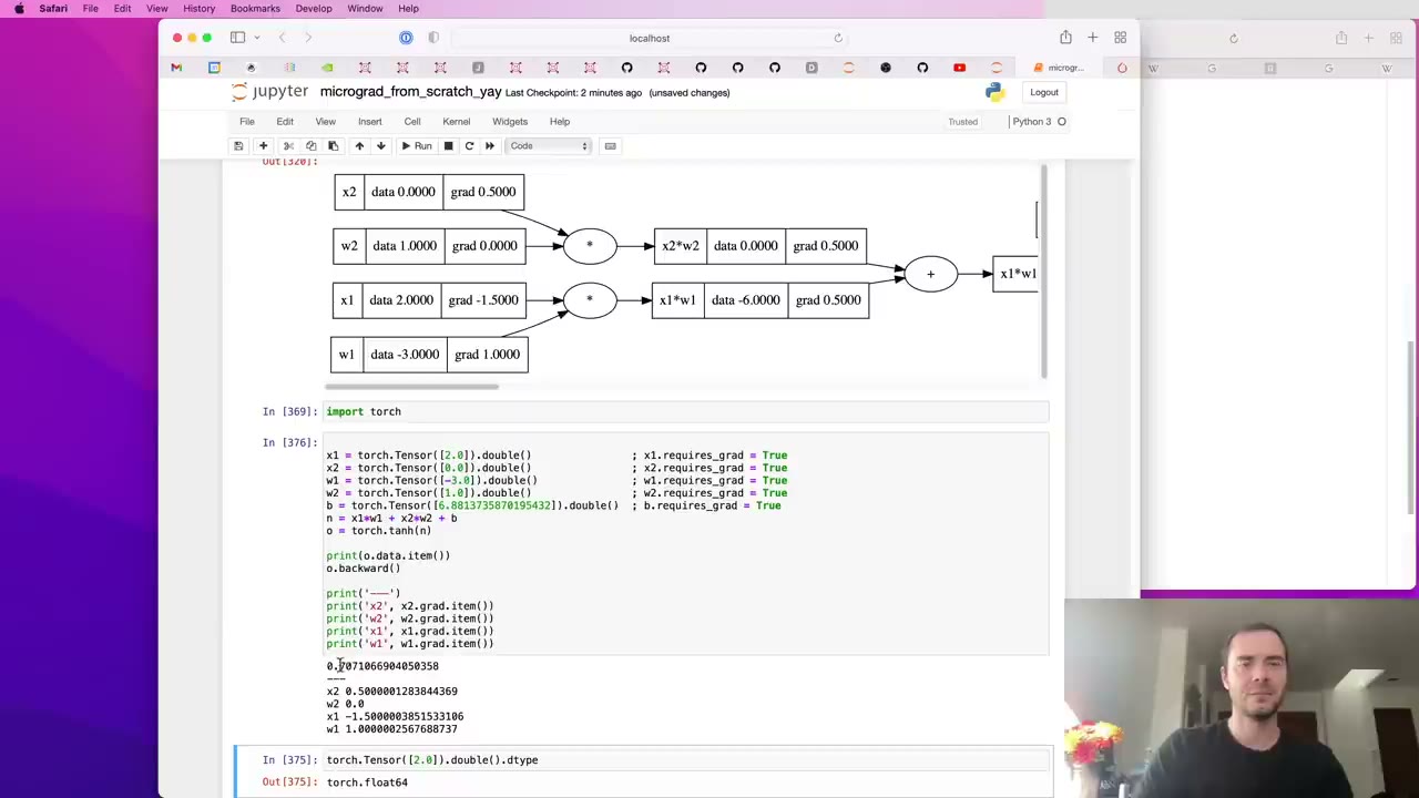 1:42:55
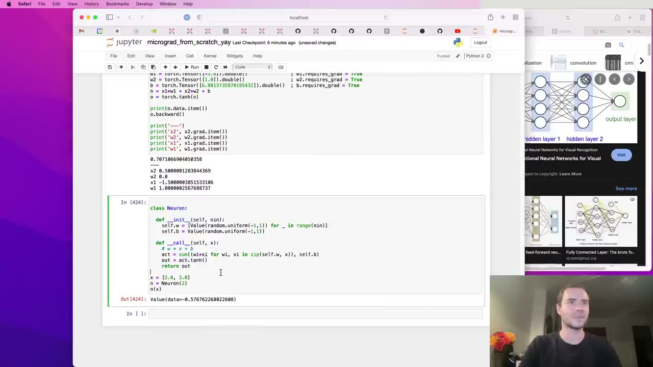 1:48:16
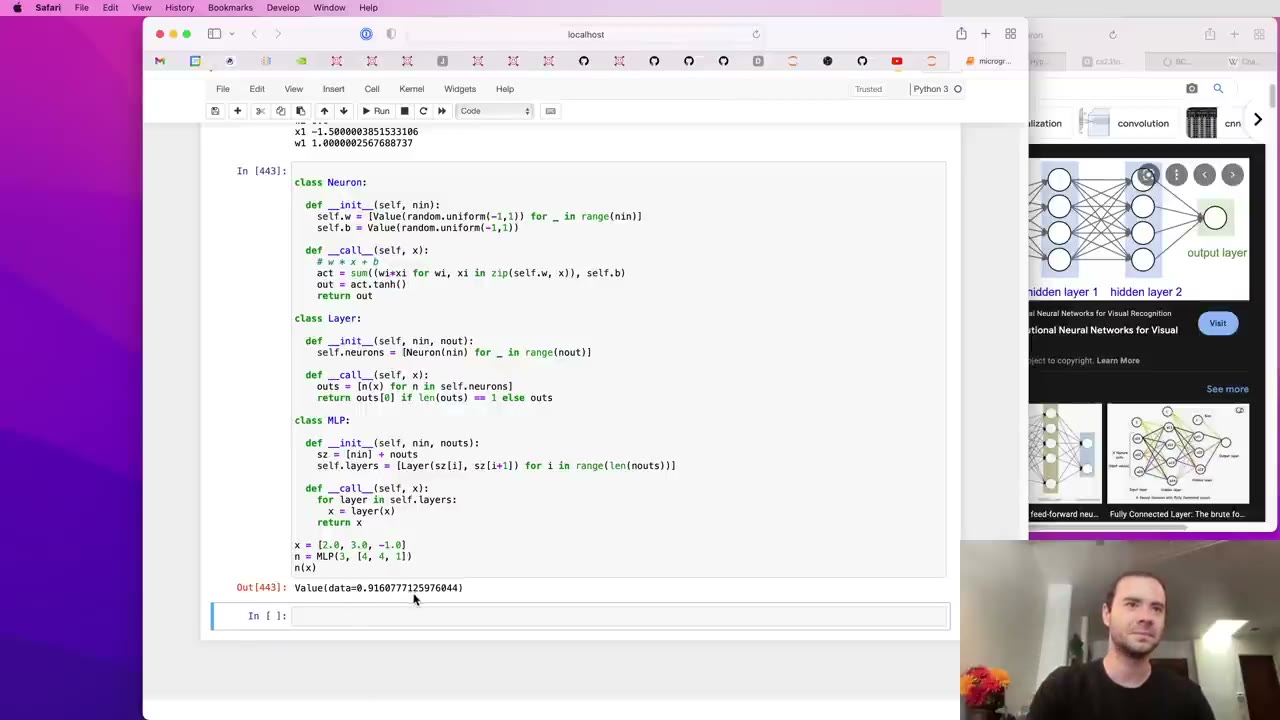 1:50:27
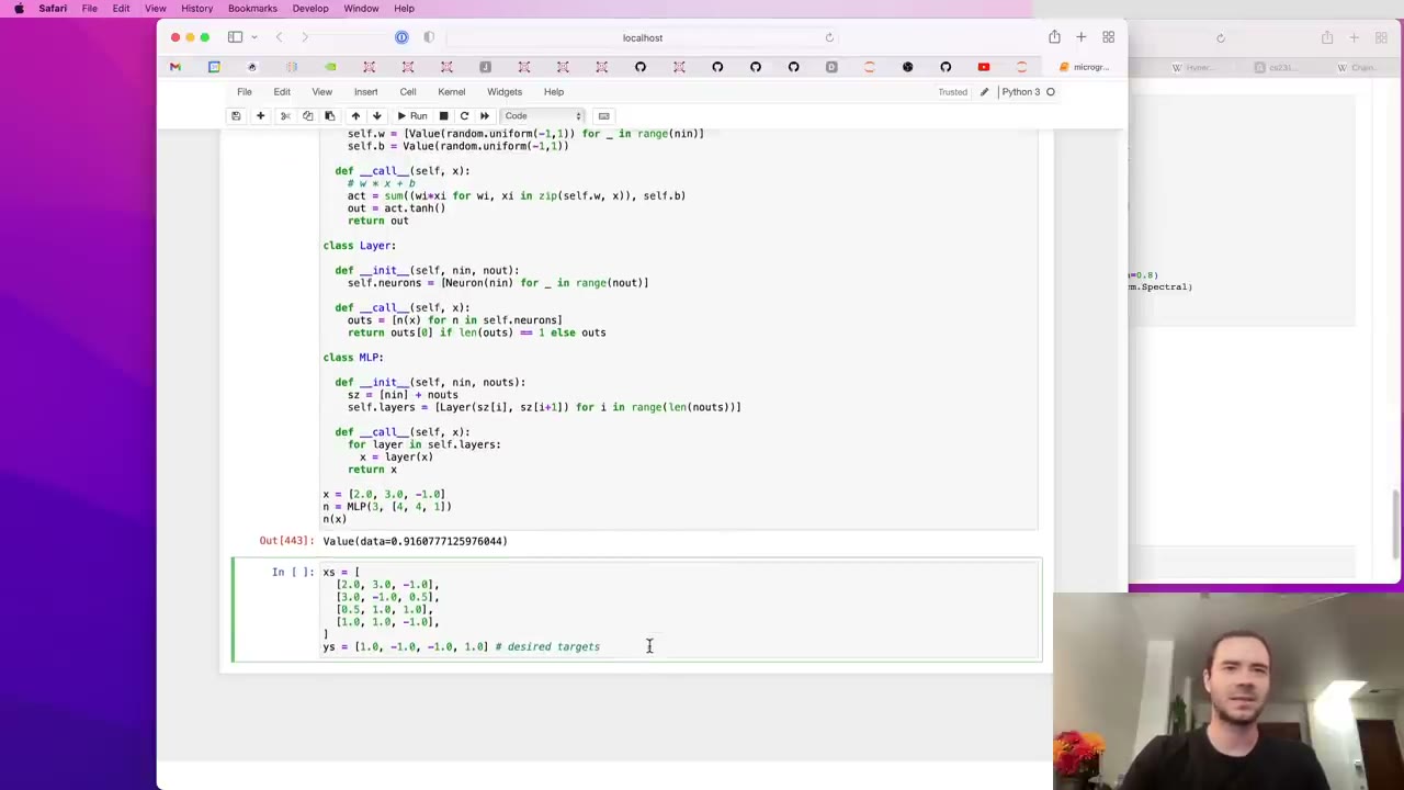 1:51:07
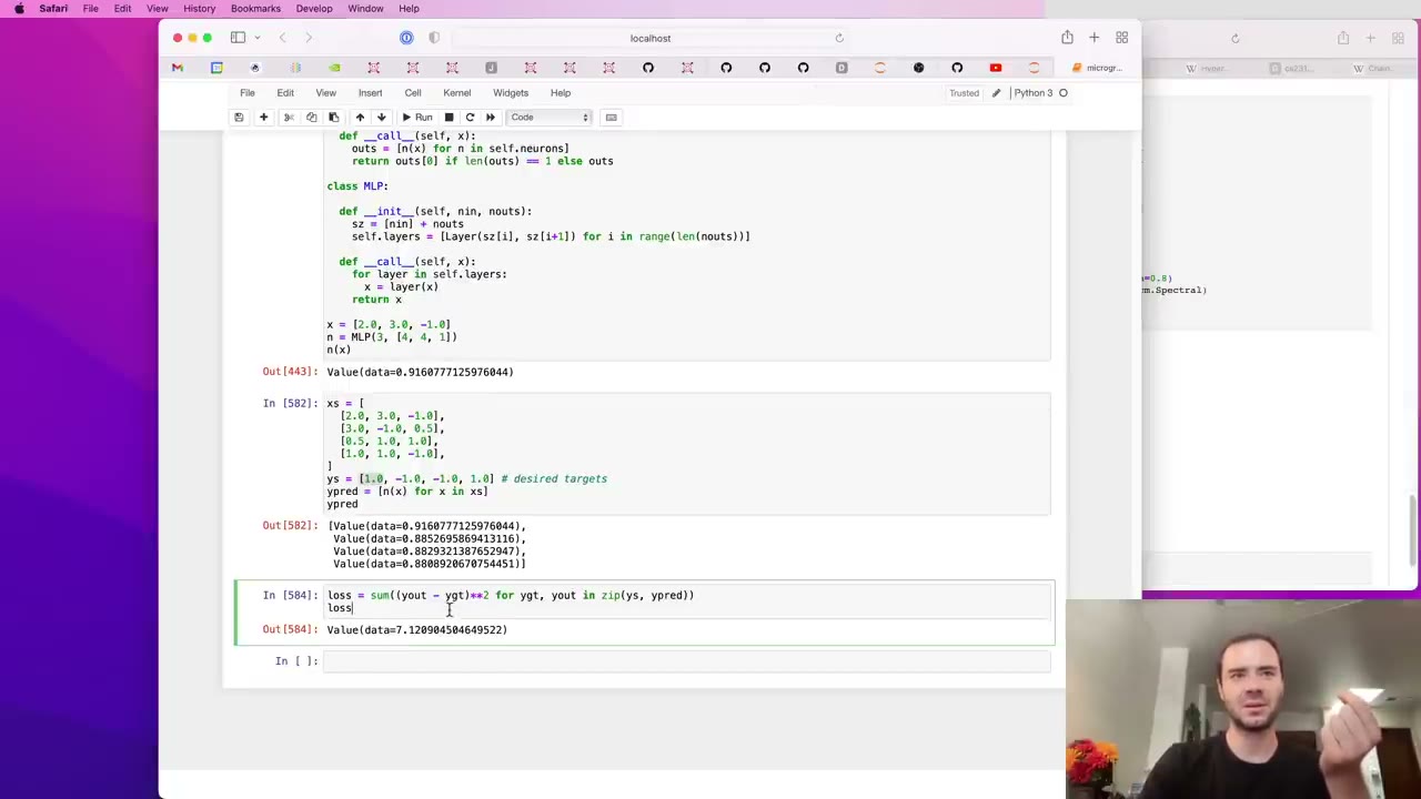 1:54:49
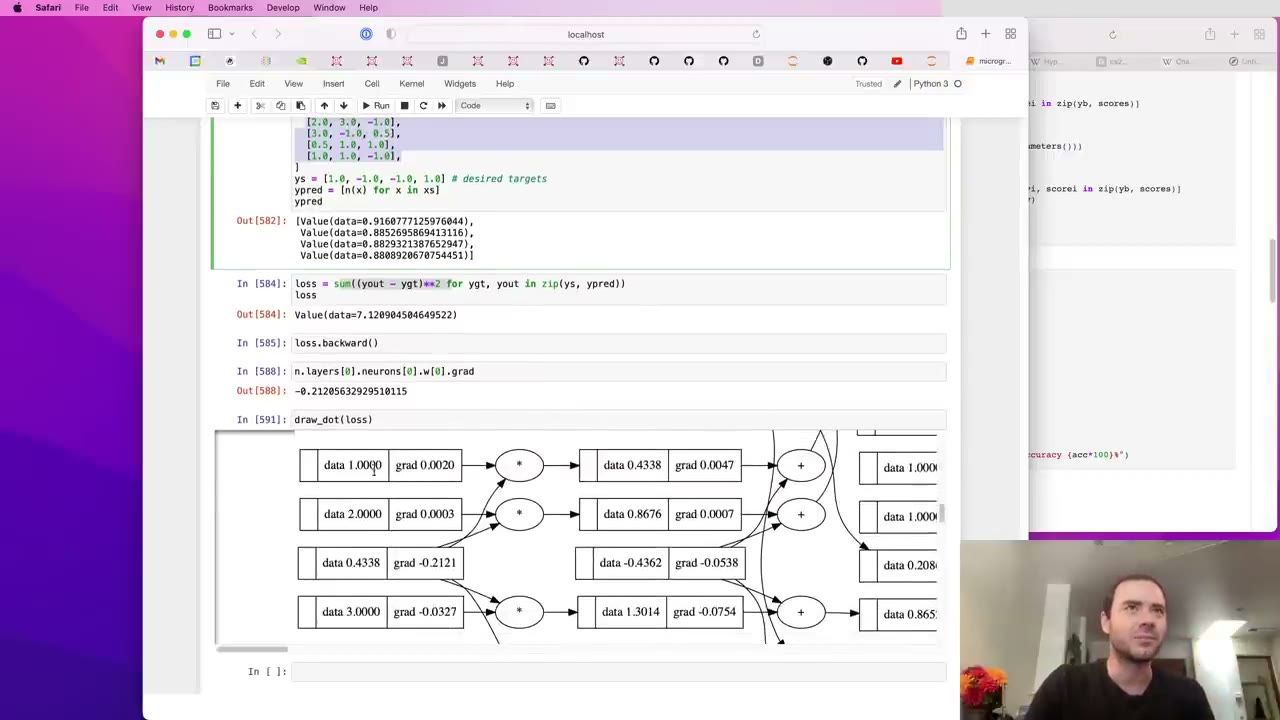 1:57:19
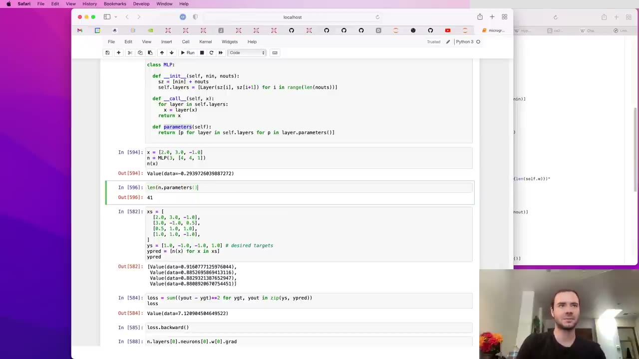 2:01:10
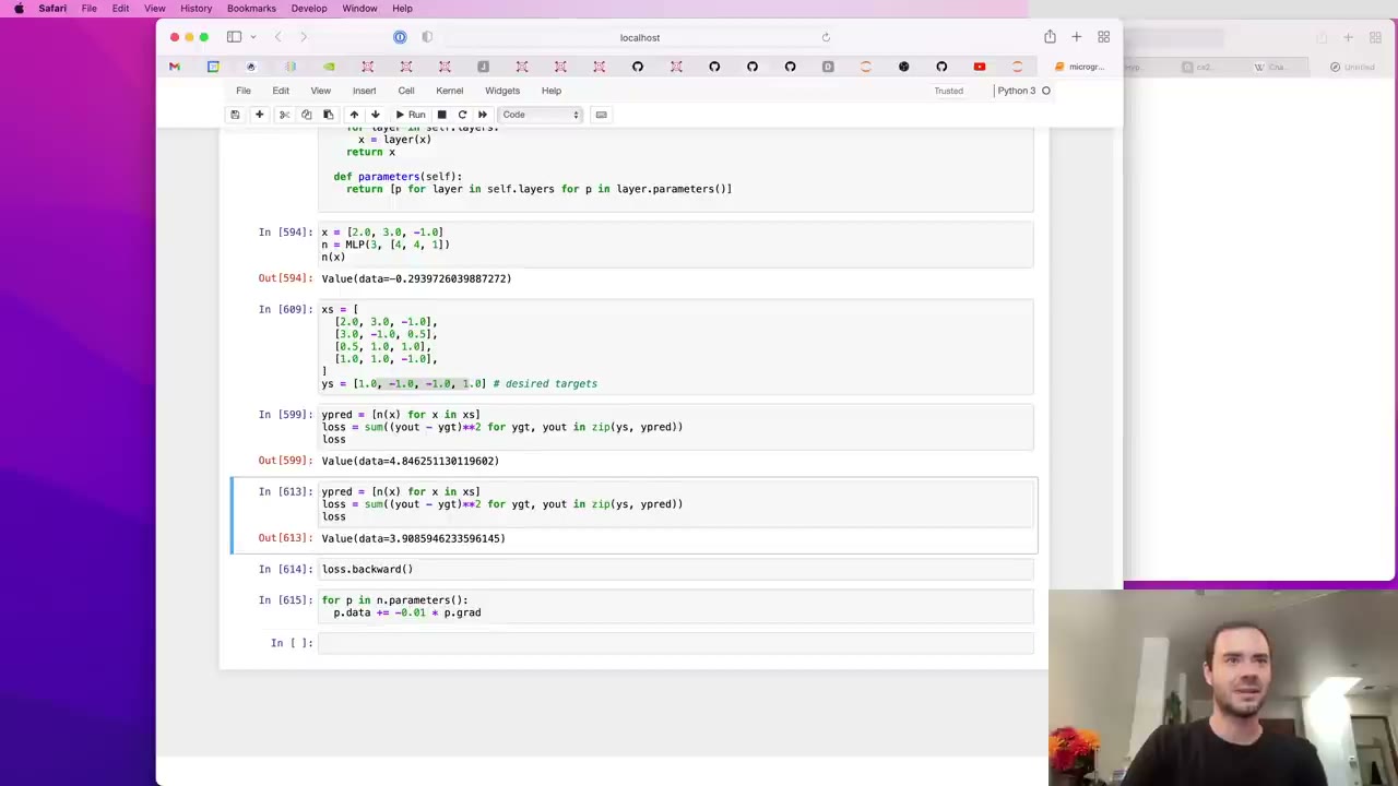 2:05:46
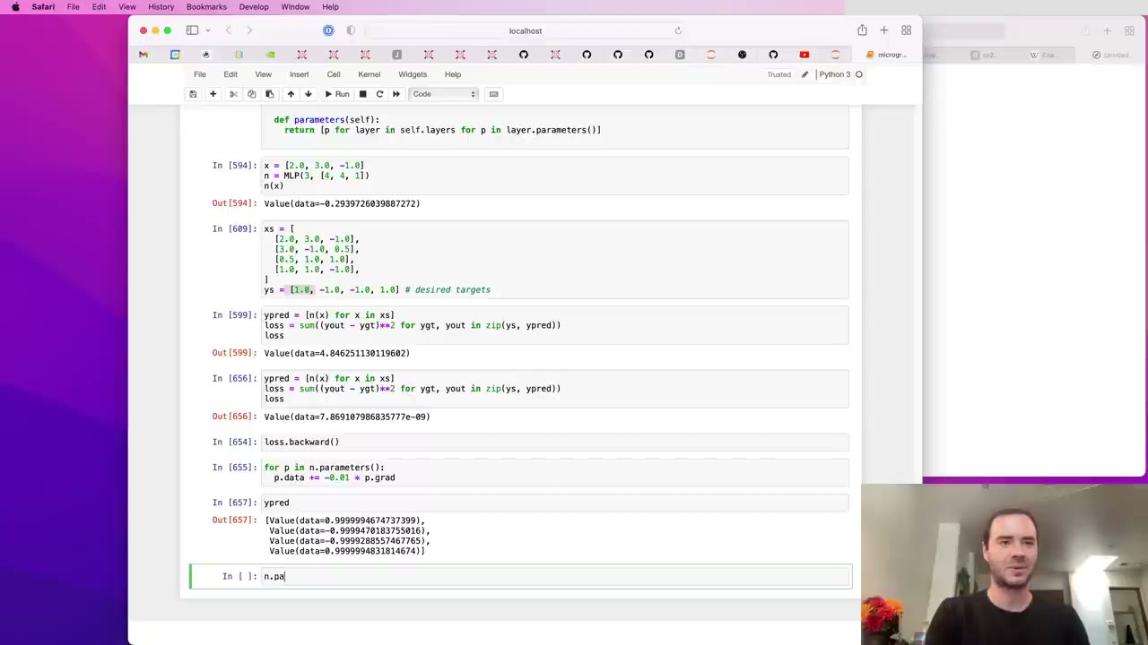 2:08:20
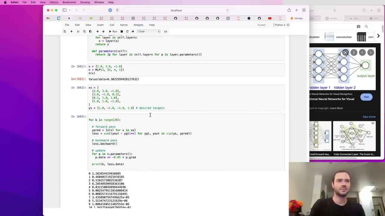 2:10:02
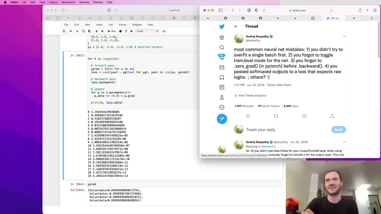 2:10:55
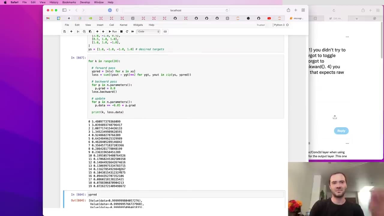 2:12:40
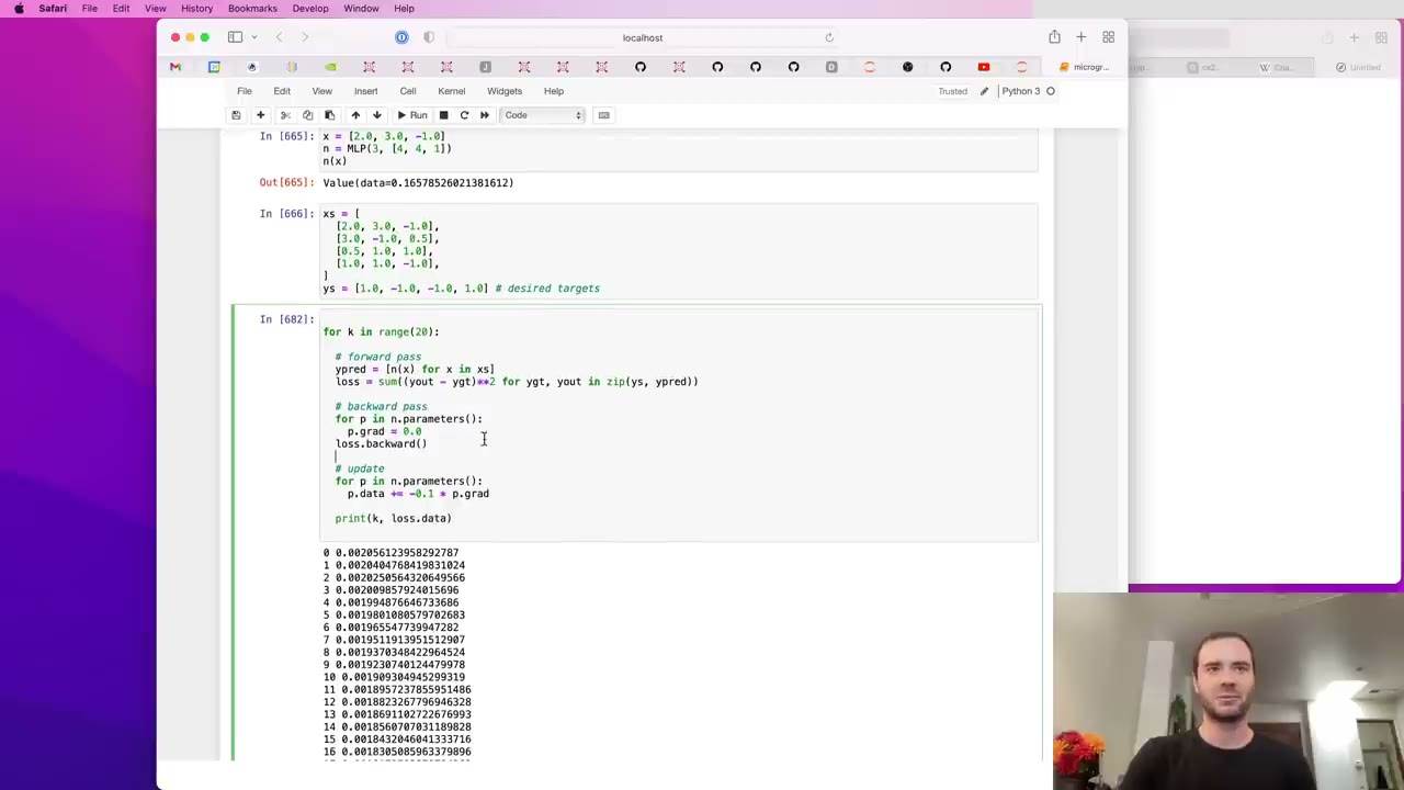 2:16:21
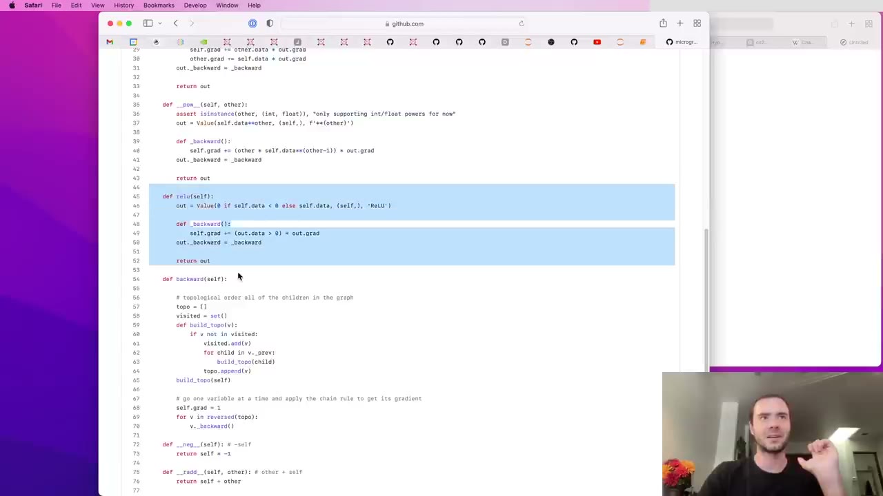 2:17:28
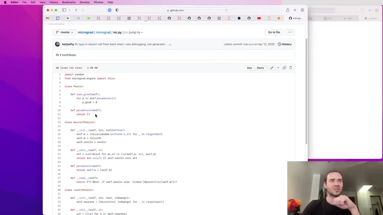 2:18:20
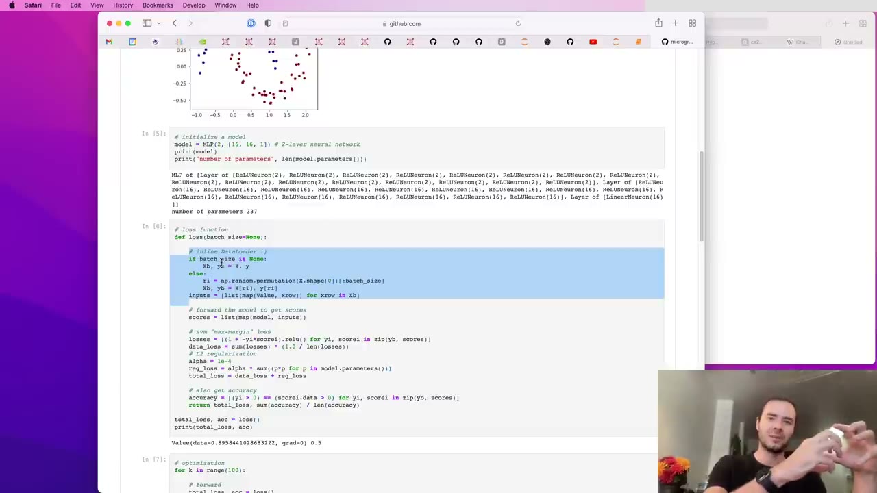 2:19:40
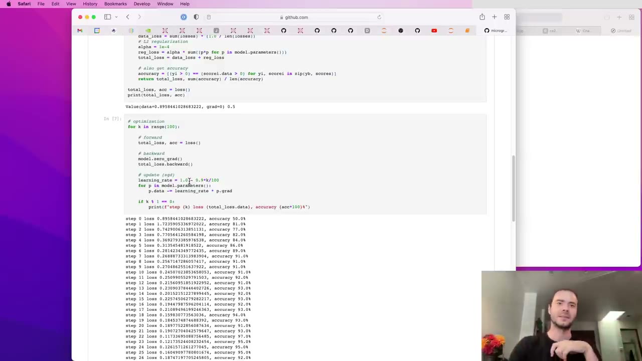 2:20:52
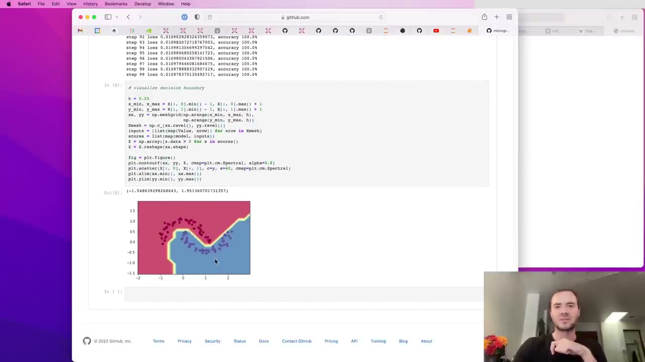 2:20:55
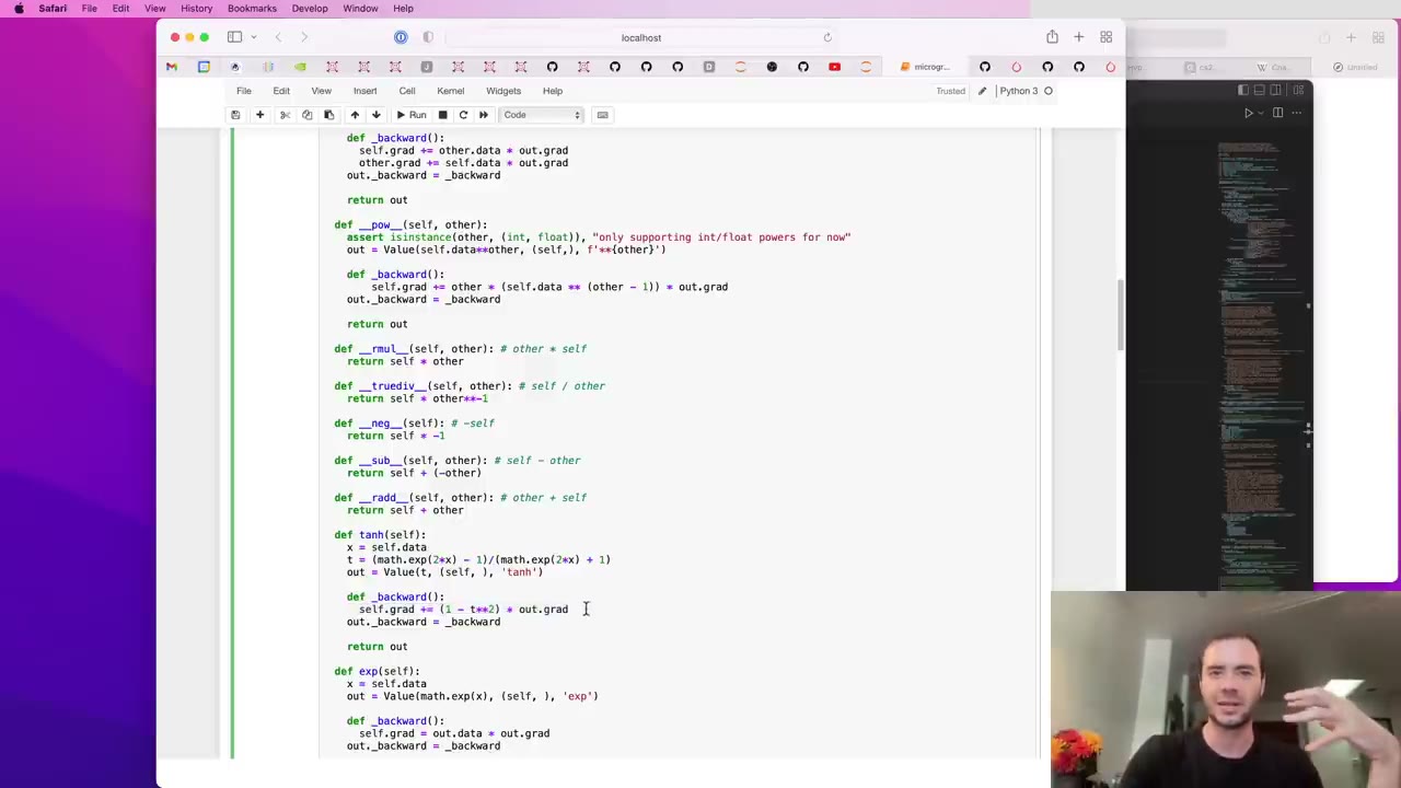 2:21:15
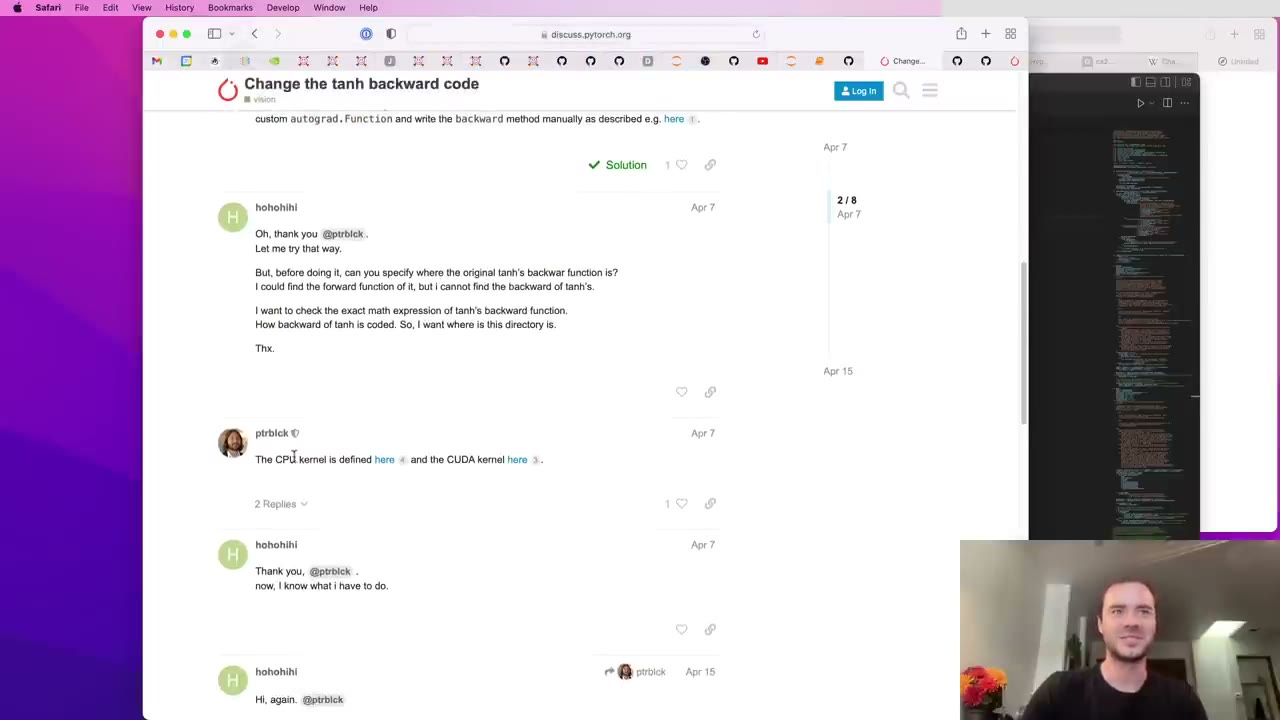 2:22:24
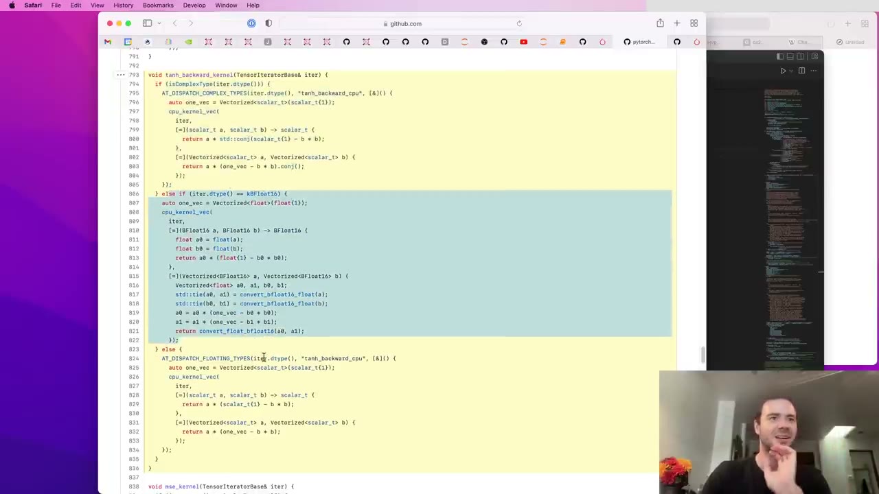 2:22:52
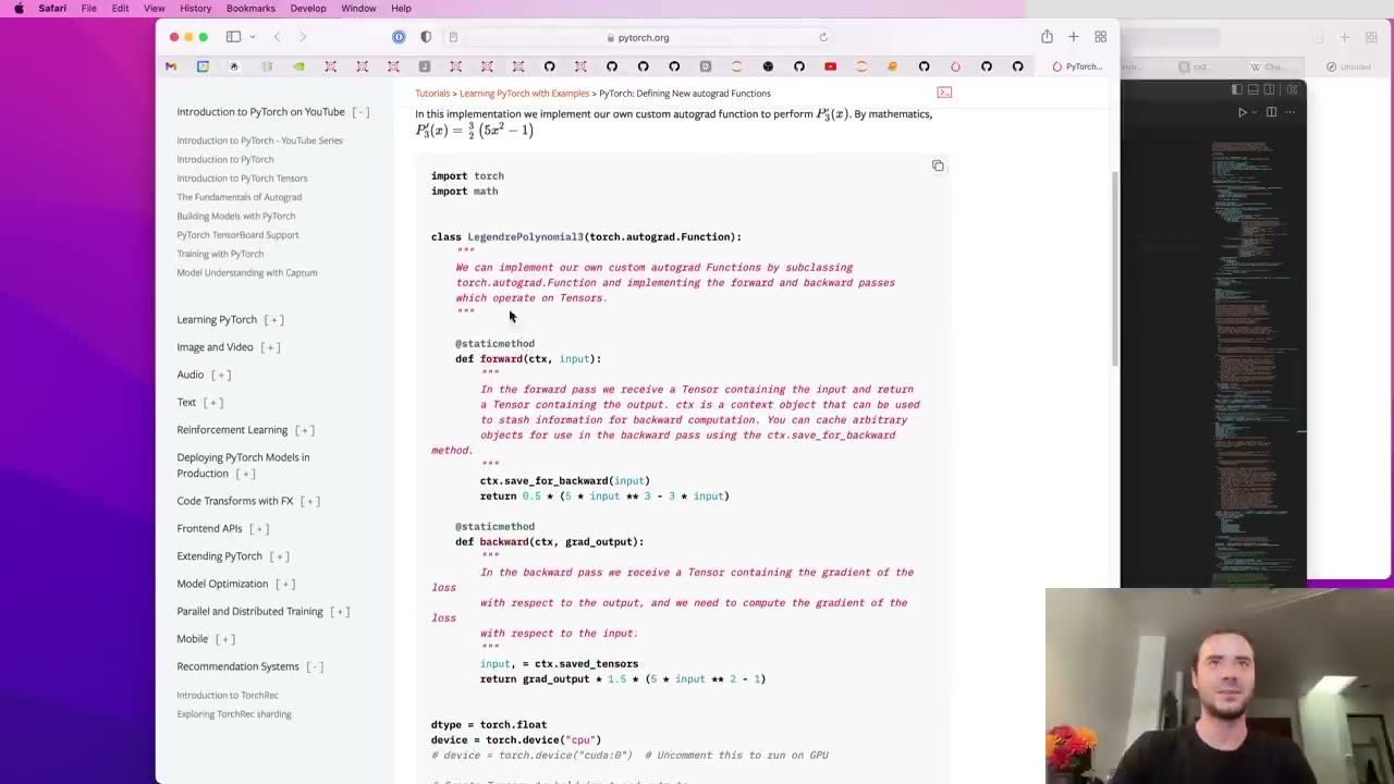 2:24:00
Watch the video (146 min)
Watch the original video on YouTube
The first lecture of Andrej Karpathy’s Neural Networks: Zero to Hero series starts from an empty Jupyter notebook and ends with a trained neural network, with nothing hidden in between. Along the way you build micrograd, Karpathy’s small autograd engine: a Value class that remembers how every number was computed, plus a backward pass that walks that record in reverse and applies the chain rule at each step. On top of it sit a neuron, a layer and a multi-layer perceptron, trained with plain gradient descent on four examples. The lecture’s central claim is that this is the whole idea behind neural network training, and that everything a production library adds is efficiency. It is the longest lecture in the series and the only one that works on single numbers instead of tensors. This is the first lecture, so there is no previous one; next comes Lecture 2: makemore, and the full series map is on the series index.
Key takeaways
- A neural network is just a mathematical expression (4:42). It takes data and weights as inputs and produces predictions or a loss. Backpropagation works on any such expression; networks are one use of it.
- A derivative is a sensitivity you can measure (10:55). Nudge an input by a tiny h, see how far the output moves, divide by h. Every gradient in the lecture is checked this way.
- The chain rule turns local derivatives into global ones (43:44). Each node only knows how its own inputs affect its own output; multiplying that by the gradient arriving from above gives the gradient with respect to the final output.
- A node can be as big or as small as you like (58:15). A plus, a times, or a whole tanh can each be one operation, as long as you can write its local derivative.
- Backward needs a topological order (1:18:01). A node’s gradient is complete only after everything that depends on it has passed gradient back, so you sort the graph and walk it in reverse.
- Gradients must accumulate (1:24:54). When a value feeds into more than one place, the contributions add up, so
_backwarduses+=rather than=. - Training is forward, zero grad, backward, update, repeated (2:11:25). Forgetting to zero the gradients is a classic bug that a toy problem can hide.
- Scale changes, principles don’t (2:15:40). A GPT-style model has vastly more parameters and a different loss, but the same value-gradient-descent loop.
Chapter notes
0:01 – 8:18 What micrograd is and why scalars
Karpathy introduces micrograd as an autograd (“automatic gradient”) engine whose job is backpropagation: efficiently computing the gradient of a loss with respect to a network’s weights, so the weights can be tuned to make the loss smaller. He calls backpropagation the mathematical core of libraries like PyTorch and JAX.
The README example shows the interface (1:34): two inputs, -4 and 2, wrapped in Value objects and run through a made-up expression with addition, multiplication, powers, ReLU and division. Reading .data on the output gives the forward pass (24.7); calling .backward() fills in .grad on every node (3:09), and a.grad of about 138 says how steeply the output rises if a is nudged upward.
g.backward(), then read the output and the gradients of a and b. The lecture is about making these few lines work.Two framing points come before any code. Neural networks are a particular kind of mathematical expression, and backpropagation does not care that they are networks (4:42). And micrograd works on individual scalars, which you would never do in production; tensors pack scalars into arrays so the computer can work on them in parallel, but the math is the same (5:45). Then the claim that frames the lecture (6:46): micrograd “is what you need to train your networks and everything else is just efficiency.” The repo has just two files that matter, engine.py (around 100 lines) and nn.py (7:17).
engine.py for the autograd engine, nn.py for the network library, and an empty __init__.py.8:18 – 18:48 What a derivative actually measures
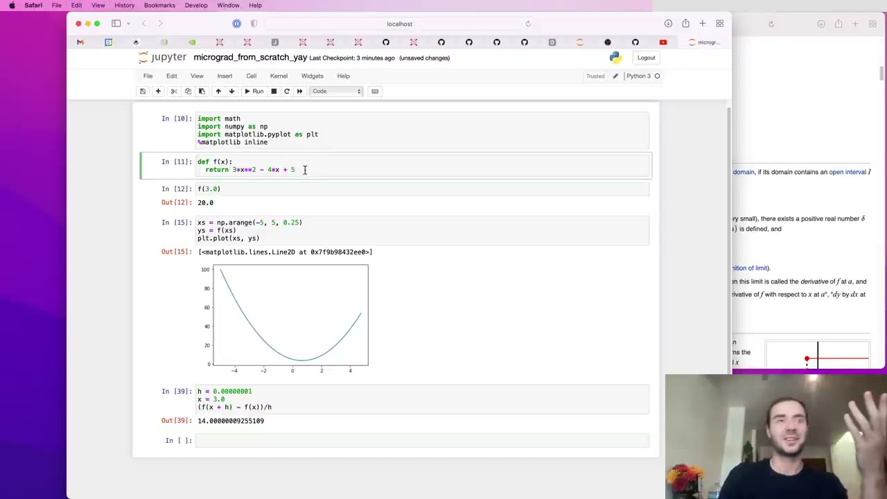
Instead of symbolic calculus, which nobody does for a network with tens of thousands of terms (9:51), the lecture works from the definition. Take f(x) = 3x² − 4x + 5, plot it as a parabola, and estimate the slope at x = 3 as (f(x + h) − f(x)) / h with h = 0.001 (11:26). The answer is close to 14, matching 6x − 4. Making h too small eventually breaks the estimate because floating-point numbers have finite precision (12:28). At x = −3 the slope is negative, and near x = 2/3 it is zero.
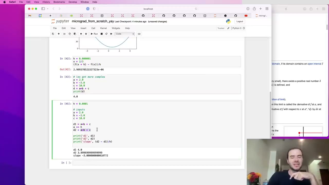
Then a function of three inputs, d = a·b + c with a = 2, b = −3, c = 10 (14:03). Bumping each input in turn gives slopes of −3 for a (the value of b), 2 for b (the value of a) and 1 for c. Karpathy asks the viewer to predict the sign before each run, which is the habit worth copying: decide whether the output should go up or down before you look.
18:48 – 29:08 The Value object and the expression graph
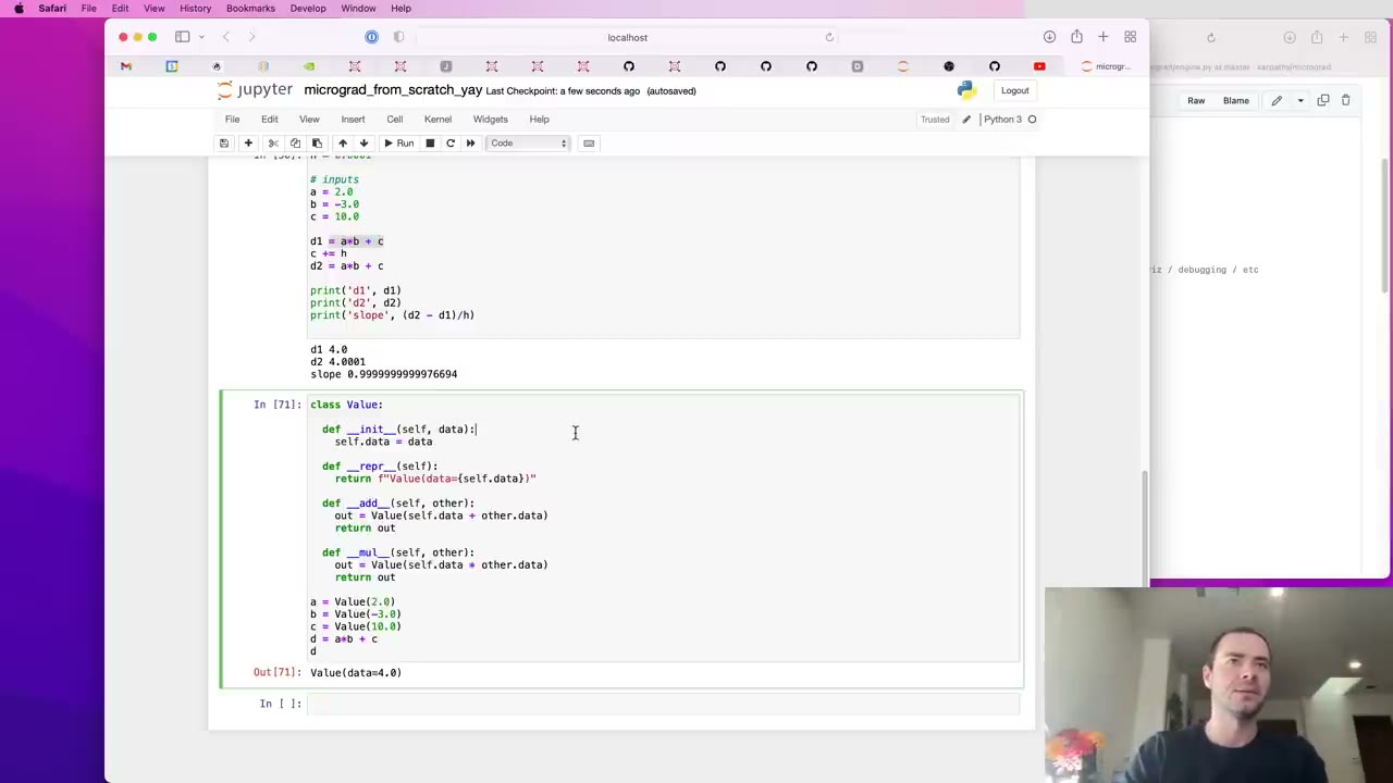
The data structure starts tiny: a Value class that wraps one number (19:19). Python’s double-underscore methods let a + b and a * b produce new Value objects, and __repr__ gives readable printing (21:55).
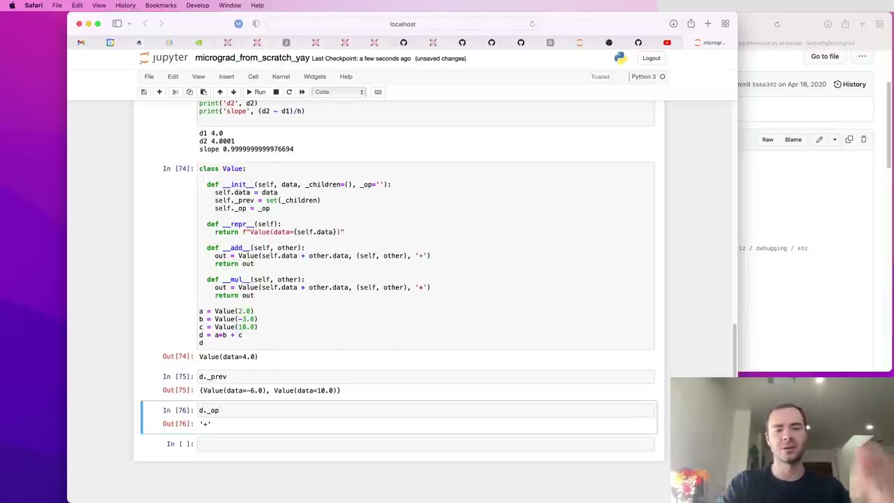
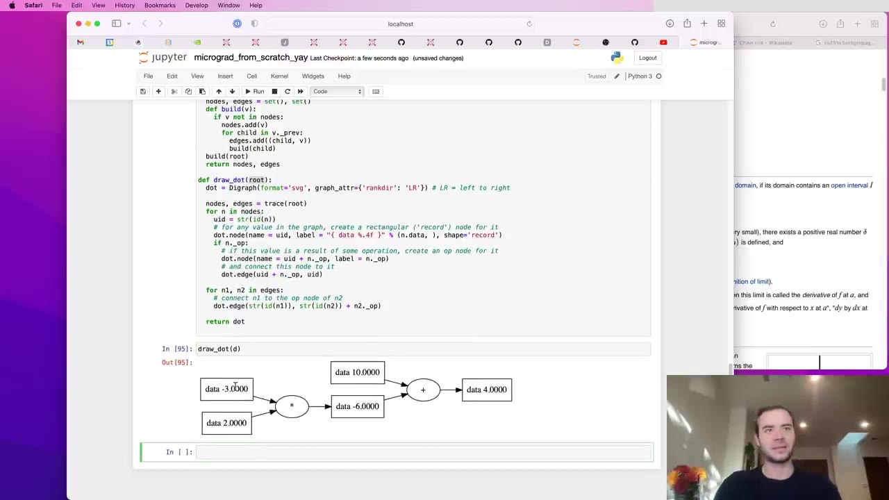
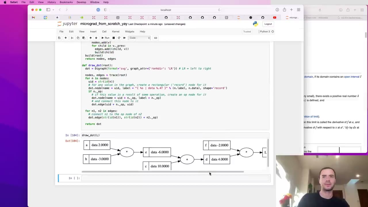
__add__ and __mul__ defined, a*b + c on Value objects works and prints through __repr__.What turns this into an engine is bookkeeping. Each result stores the values that produced it in _prev (passed in as a _children tuple, kept as a set; Karpathy thinks the set was for efficiency) and the operation that produced it in _op (22:56). With that, a chain of values is a full expression graph. A pasted draw_dot helper renders it with Graphviz, adding fake operation nodes so the picture reads well (25:00). Labels are added, and the running example becomes e = a·b, d = e + c, L = d·f with f = −2, so L = −8 (28:07).
_prev and the '+' that produced it in _op.
draw_dot adds for readability.
29:08 – 37:57 Manual backprop, the first steps
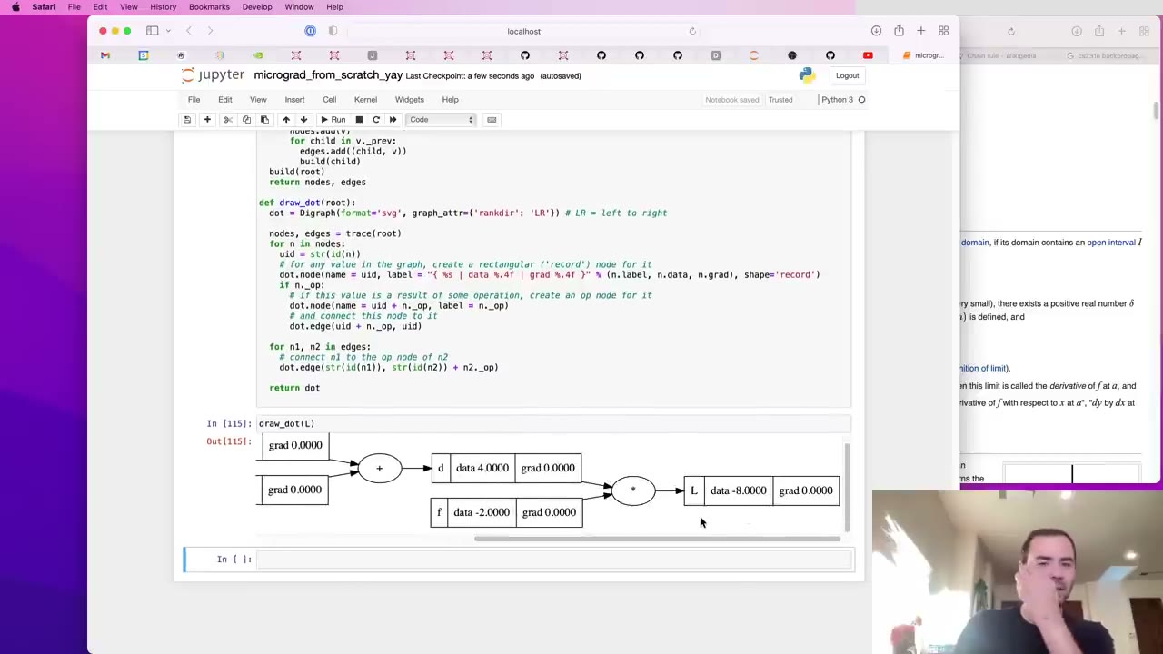
Backpropagation computes, for every node, the derivative of the final output L with respect to that node (29:39). In a real network the nodes you care about are the weights; the inputs are data, which you are not going to change. Each Value gets a grad field starting at 0.0, meaning no effect on the output by default (30:41).
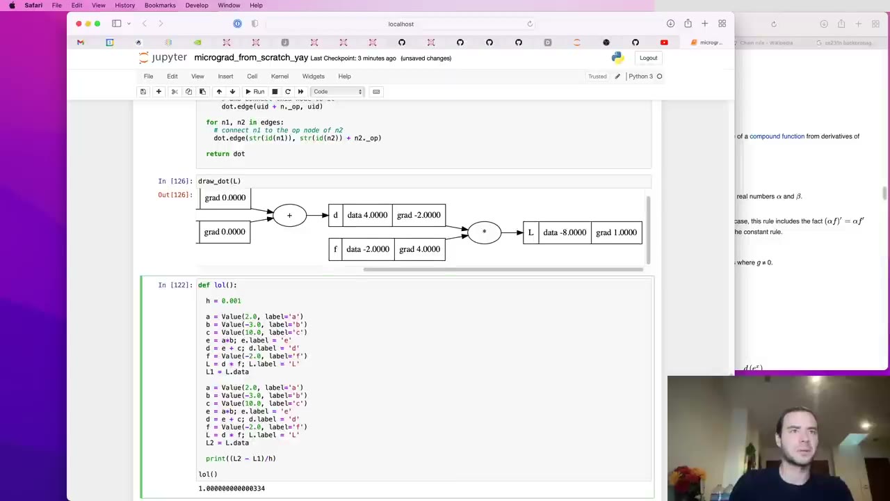
grad field added, each node shows its gradient, still zero because nothing has been backpropagated yet.The base case is L.grad = 1. For L = d·f, Karpathy derives from the limit definition that dL/dd = f and dL/df = d (34:51), so d.grad = −2 and f.grad = 4. Each claim is confirmed by bumping that one value by h inside a throwaway function and measuring the change in L. He names this an inline gradient check (37:26): comparing derived gradients with numerical estimates.
lol() cell underneath is the throwaway function used for numerical checks.37:57 – 52:34 The chain rule, the crux of it all
Karpathy flags the next node as the one to understand (37:57): if you get dL/dc, you get backpropagation. The plus node that made d knows only its local derivatives, dd/dc = 1 and dd/de = 1 (40:38). It knows nothing about the rest of the graph. The chain rule combines that local knowledge with dL/dd, already computed, by multiplying them (41:41). He prefers Wikipedia’s car-bicycle-walker version: if a car is twice as fast as a bike and the bike four times as fast as a walker, the car is eight times as fast (43:14).
Two patterns fall out:
| Node | Local derivative | What it does to the incoming gradient |
|---|---|---|
| a + b | 1 for each input | Routes it unchanged to both inputs (45:17) |
| a × b | the other input’s value | Scales it by the other factor (47:52) |
So c and e both get −2, then a.grad = −2 × −3 = 6 and b.grad = −2 × 2 = −4, each verified numerically (49:59). The summary sentence is worth memorizing: backpropagation is a recursive application of the chain rule, backwards through the computation graph (50:30).
A quick demonstration closes the section (51:01). Nudging every leaf a small step (0.01) in the direction of its gradient and re-running the forward pass moves L from −8 to about −7. That is one step of optimization, done by hand.
52:34 – 1:01:53 A neuron, and tanh as a single operation
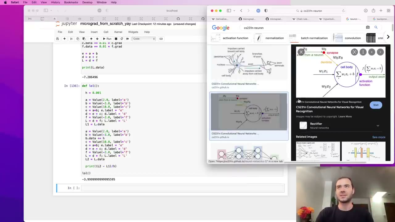
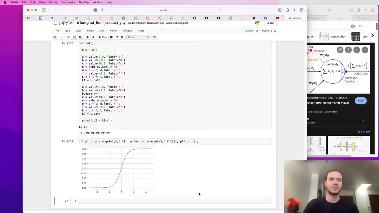
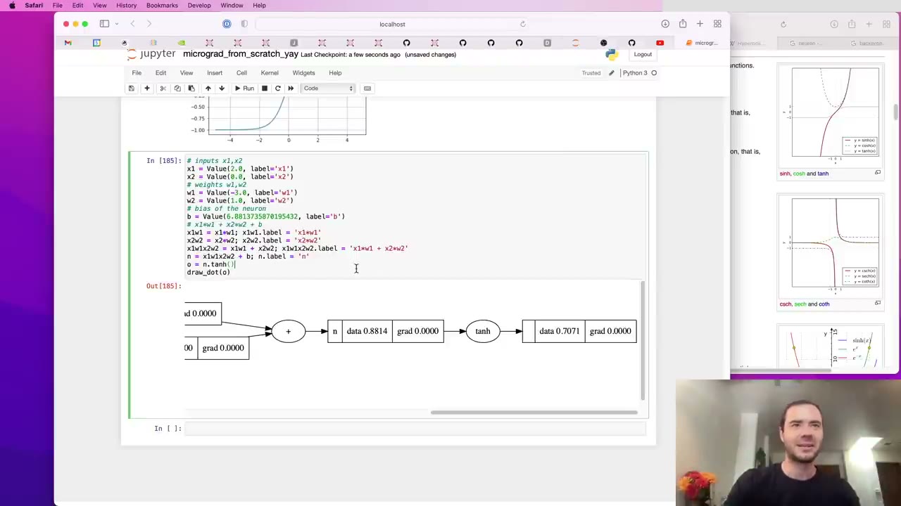
The next example is closer to a real network: one neuron (52:34). Its simple mathematical model multiplies each input x by a weight w, sums the products, adds a bias b (the neuron’s “trigger happiness”), and passes the result through a squashing activation such as tanh, which maps any input into the range −1 to 1 (54:38).
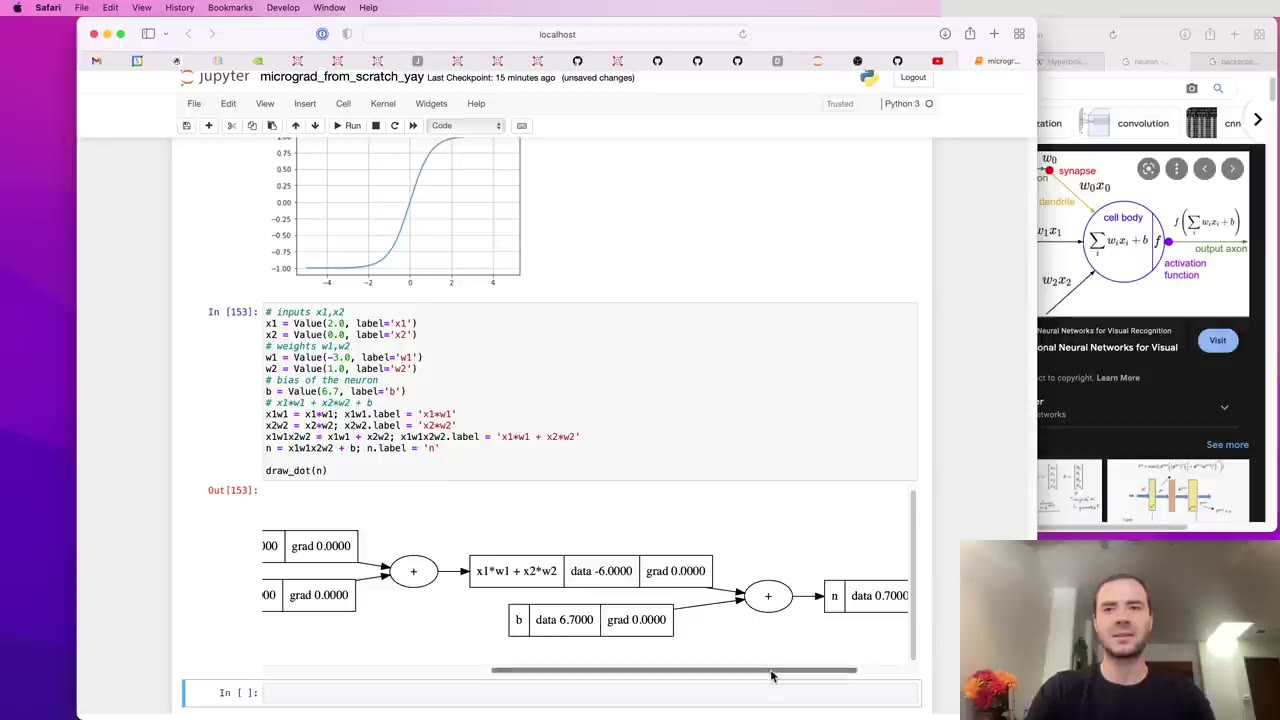
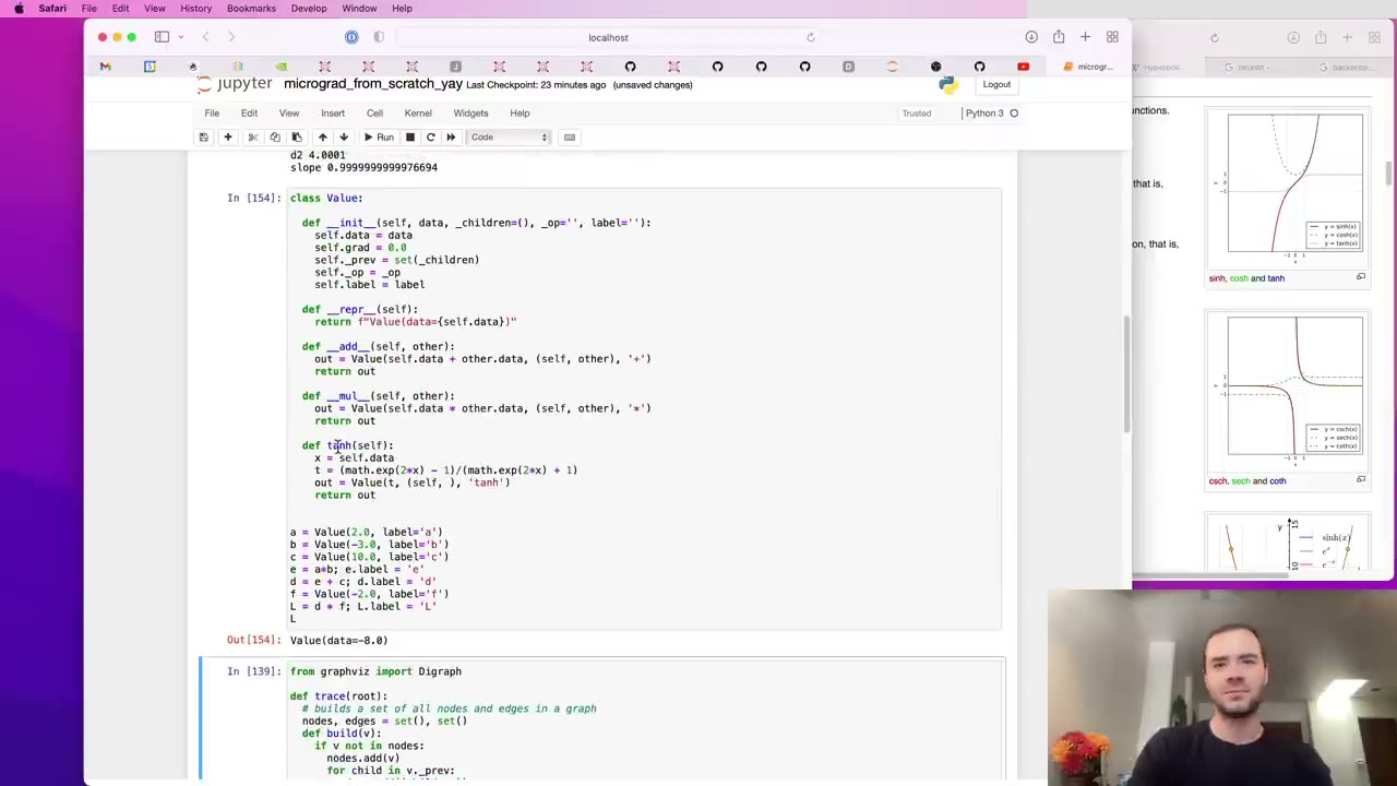
Built step by step with two inputs, the neuron needs a tanh operation, which plus and times alone cannot build (57:12). Karpathy could implement exponentiation and assemble tanh from pieces, but deliberately implements tanh as one node instead (58:15). The point: an operation can sit at any level of abstraction, as long as you know its local derivative. He then sets the bias to an odd-looking 6.88… so the numbers come out round: the raw sum is about 0.88 and the output is 0.7071 (1:01:22).
1:01:53 – 1:08:59 Backprop through the neuron by hand
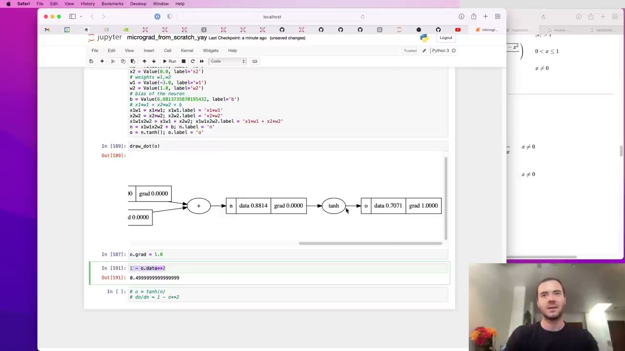
Starting from o.grad = 1, the tanh step needs d(tanh n)/dn = 1 − tanh²(n), which is just 1 − o² because o is already computed (1:03:26). With o ≈ 0.7071 that is 0.5. The two plus nodes pass 0.5 through untouched (“pluses are my favorite”), and the times nodes swap in the other factor (1:06:23).
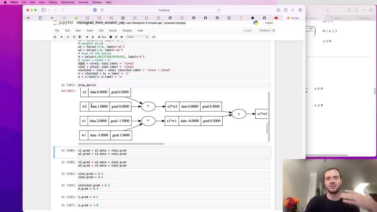
The results: w2.grad = 0 because its input x2 is 0, so wiggling w2 cannot change the output; x2.grad = 0.5; x1.grad = −1.5; w1.grad = 1 (1:08:29). Read as advice, w1 is the weight to increase if you want this neuron’s output to rise.
1:08:59 – 1:17:30 Codifying it: _backward closures
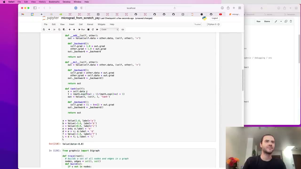
Manual backprop is “obviously ridiculous” for anything bigger, so each operation now records how to push gradient back to its inputs (1:09:31). Every Value gets a _backward function, empty by default (leaf nodes have nothing to do). When __add__, __mul__ or tanh creates an output, it defines a closure that multiplies the output’s gradient by the local derivative and stores the result in the inputs’ .grad, then attaches that closure to the output (1:10:35).
Calling these by hand in the right order, after setting o.grad = 1, reproduces the earlier numbers (1:17:00). Karpathy leaves a mistake in on purpose (1:14:56): writing out._backward = _backward() calls the function and stores its return value, None, instead of storing the function.
out._backward held None.
_backward by hand, from the output back, reproduces the manual gradients.1:17:30 – 1:22:15 Topological sort and backward()
The remaining manual step is the order of those calls. A node’s _backward must not run until every node that uses it has already passed gradient back (1:17:30). The tool is topological sort, which lays out a directed acyclic graph so all edges point one way (1:18:01). His version is a short recursive function: visit a node once, recurse into its children, then append the node, so a node lands in the list only after all its children (1:19:02).
Walk the list in reverse, calling _backward on each node, and every gradient is filled in. That logic then moves into a public backward() method on Value, which builds the order from self, sets self.grad = 1.0 and runs the loop (1:21:13).
Value.backward(), so one call fills every gradient.1:22:15 – 1:26:28 The bug: using a value twice
Karpathy then shows a bug that the examples so far hid (1:22:15). With b = a + a, the gradient of b with respect to a should be 2, but the code gives 1. The plus node’s self and other are the same object, so the second assignment overwrites the first. A bigger example in which a and b each feed two different nodes fails the same way (1:24:23).
The fix comes from the multivariable chain rule: when a value is used in several places, the gradients from each use add up. So every _backward switches from = to += (1:24:54), which works because gradients start at zero.
+= in every _backward, the contributions add up and both examples come out right.Our note: this one-character change explains a PyTorch habit later in the series. Because gradients accumulate by design, something has to reset them before each new backward pass. The lecture’s final bug comes from exactly that.
1:26:28 – 1:39:28 More operations, and tanh rebuilt from parts
To prove that implementing tanh as one node was a choice, not a necessity, Karpathy rebuilds it from smaller operations, adding several along the way (1:26:59):
- Plain numbers.
a + 1failed because 1 has no.data;__add__and__mul__now wrap non-Valuearguments (1:28:33). - Reversed operands.
2 * afails because Python first asks the integer, so__rmul__handles it by swapping the order (1:29:36). - exp. The derivative of eˣ is eˣ, which the output already holds (1:31:09).
- Powers and division. Rather than division directly, he implements x raised to a constant k with the power rule, k·x^(k−1), and defines a / b as a · b⁻¹ (1:32:11).
- Subtraction. Negation is multiplying by −1, and a − b is a + (−b) (1:35:46).
a + 1 works.
2 * a fails because Python asks the integer first; __rmul__ is the fallback that fixes it.
+=; the lecture notebook in nn-zero-to-hero has the fix.
__truediv__, which multiplies by b to the power −1.
Then tanh becomes (e²ˣ − 1) / (e²ˣ + 1) in the neuron (1:36:49). The graph gets much longer, but the forward value and all four leaf gradients match the single-node version (1:37:53). The lesson he draws is that “composite” versus “atomic” is a fake distinction (1:38:56): any piece with a forward pass and a local derivative can be a node.
1:39:28 – 1:43:40 The same neuron in PyTorch
The same neuron in PyTorch shows micrograd’s design is not arbitrary (1:39:28). PyTorch works with tensors, n-dimensional arrays, so each scalar becomes a one-element tensor. Two details: he casts to double so the precision matches Python floats (PyTorch defaults to float32), and he sets requires_grad = True because leaf tensors don’t track gradients by default (1:41:03). After o.backward(), .item() pulls numbers out and gives 0.7071 forward, then 0.5, 0, −1.5 and 1 (1:42:36). Micrograd is PyTorch’s autograd restricted to single-element tensors; PyTorch’s advantage is speed.
1:43:40 – 1:51:02 Neuron, Layer and MLP
Now the network library, modeled on PyTorch’s nn modules (1:44:12). A Neuron takes its number of inputs, creates a random weight between −1 and 1 for each plus a bias, and in __call__ computes the weighted sum plus bias through tanh (1:46:50). Passing self.b as the start value of sum saves a separate addition.
A Layer is a list of independent neurons all fed the same inputs (1:47:55). An MLP takes the input size and a list of layer sizes and chains layers so each feeds the next (1:48:58). The lecture’s network is MLP(3, [4, 4, 1]): three inputs, two hidden layers of four, one output. A small convenience makes a one-neuron layer return a bare value rather than a list (1:50:00), and draw_dot on the output now shows a large graph.
1:51:02 – 2:08:41 A loss, parameters and gradient descent by hand
The dataset has four three-number inputs with targets 1, −1, −1, 1, a tiny binary classifier (1:51:02). Untrained predictions are far off. To judge the whole network with one number, the loss sums, over the four examples, the squared difference between prediction and target (1:52:34). Squaring discards the sign, so the loss is zero only when every prediction hits its target. It starts around 7.
Calling loss.backward() fills a gradient into every weight (1:54:38). The graph is now huge: four forward passes plus the loss on top (1:56:10). The inputs get gradients too, but data is fixed, so only the weights and biases matter. A parameters() method on each class collects them, 41 in total (2:00:55).
loss.backward() the graph is too big to view at once, but every weight in it now has a gradient.
parameters() gathers every weight and bias: 41 for this network.The update needs care with its sign (2:02:29). The gradient points toward higher loss, so each parameter moves by a small step times the negative gradient. After a few rounds of forward, backward and update by hand, the loss falls from 4.84 to 4.36, 3.9, 3.66 and on (2:05:34). A bigger step speeds things up, then overshoots and briefly blows up before landing at a near-zero loss (2:07:08). Karpathy calls setting the learning rate a subtle art: too low is slow, too high is unstable.
Our note: Karpathy calls this the mean squared error, but the code adds the squared errors without dividing by four. That only rescales the loss and its gradients, which in effect changes the step size.
2:08:41 – 2:14:06 The training loop and the zero_grad bug
The steps go into a proper loop of 20 iterations, with a learning rate of 0.05, between 0.01 (too slow) and 0.1 (too jumpy) (2:08:41). It converges nicely, and then Karpathy admits there is a bug he has made “for the 20th time” (2:10:23), number three on a list of common neural net mistakes he once tweeted: forgetting to zero the gradients before backward.
loss.backward().
Because every _backward adds into .grad, the gradients from each iteration piled on top of the last. The fix is to set p.grad = 0.0 for every parameter before loss.backward() (2:11:56), the same job as zero_grad in PyTorch. Descent is now slower but correct. The buggy version only worked because the problem is so easy that the accumulated gradients acted like an oversized step (2:12:59). His broader warning: neural nets can appear to train while full of bugs.
2:14:06 – 2:16:42 Summary: what a neural net is
Karpathy’s recap (2:14:06): a neural net is a mathematical expression of data and weights, followed by a loss designed to be low when the network does what you want. Backpropagation gives the gradient, and gradient descent follows it repeatedly downhill. This network has 41 parameters; large models have billions, and he points to GPT-style next-word prediction on internet text (2:15:40). Such models use a cross-entropy loss and fancier update rules, but the setup is the same (2:16:10).
2:16:42 – 2:20:53 A tour of the micrograd repo
To show you now understand the whole library, Karpathy walks through the repo (2:16:42). engine.py holds the Value class you have just built, with one difference: it uses ReLU rather than tanh as its nonlinearity, which he says makes no big difference (2:17:13). nn.py has the same Neuron, Layer and MLP, plus a Module parent class mirroring PyTorch’s nn.Module, with zero_grad factored into it (2:18:16). A test file checks that micrograd’s forward and backward passes match PyTorch’s.
engine.py uses ReLU in place of tanh; its backward passes gradient only where the output is positive.
nn.py: the same Neuron, Layer and MLP, under a Module base class that provides zero_grad.The demo notebook is a harder version of the lecture’s problem (2:18:47): classifying 2D points as red or blue. It adds ideas the lecture skipped. These are mini-batches (a random subset of examples per step), a max-margin loss, L2 regularization against overfitting, and learning rate decay, a step size that shrinks over training (2:20:21). It ends with the network’s decision boundary.
2:20:53 – end Inside PyTorch, and adding your own operation
For contrast, Karpathy goes looking for PyTorch’s tanh backward (2:20:53). Searching the repo returns thousands of matches; he eventually finds separate CPU and CUDA kernels, the CPU one bulked out by branches for complex numbers and bfloat16. Deep inside is the same formula as micrograd’s, 1 − t² times the incoming gradient (2:22:57). Production libraries, he notes, are meant to be used, not read.
__radd__, which the loss's sum() relies on.
The last example is PyTorch’s documentation on extending autograd, a third-order Legendre polynomial as a custom function (2:23:27). You subclass torch.autograd.Function and supply a forward and a backward. Then PyTorch can backpropagate through your function like any other building block (2:23:59). It is the same contract as a micrograd node.
Code you’ll write
These excerpts follow the lecture notebook in nn-zero-to-hero (tanh version). The full engine and network library, MIT-licensed, are in karpathy/micrograd as micrograd/engine.py and micrograd/nn.py.
The Value node with add and multiply. Each operation returns a new Value that remembers its inputs and carries a closure for its piece of the chain rule. Note the += from the accumulation fix. Built from 1:09:31, with the += fix at 1:24:54.
class Value:
  def __init__(self, data, _children=(), _op='', label=''):
    self.data = data
    self.grad = 0.0
    self._backward = lambda: None
    self._prev = set(_children)
    self._op = _op
    self.label = label

  def __add__(self, other):
    other = other if isinstance(other, Value) else Value(other)
    out = Value(self.data + other.data, (self, other), '+')
    def _backward():
      self.grad += 1.0 * out.grad
      other.grad += 1.0 * out.grad
    out._backward = _backward
    return out

  def __mul__(self, other):
    other = other if isinstance(other, Value) else Value(other)
    out = Value(self.data * other.data, (self, other), '*')
    def _backward():
      self.grad += other.data * out.grad
      other.grad += self.data * out.grad
    out._backward = _backward
    return out
tanh and power as single operations. Each needs only its forward value and local derivative: 1 − t² for tanh, the power rule for a constant exponent. tanh from 59:17, powers from 1:33:13.
  def tanh(self):
    x = self.data
    t = (math.exp(2*x) - 1)/(math.exp(2*x) + 1)
    out = Value(t, (self, ), 'tanh')
    def _backward():
      self.grad += (1 - t**2) * out.grad
    out._backward = _backward
    return out

  def __pow__(self, other):
    assert isinstance(other, (int, float)), "only supporting int/float powers for now"
    out = Value(self.data**other, (self,), f'**{other}')
    def _backward():
      self.grad += other * (self.data ** (other - 1)) * out.grad
    out._backward = _backward
return outexp, __rmul__, __truediv__ (a · b⁻¹), __neg__ and __sub__ follow the same pattern or are defined in terms of these (1:28:33). Our note: the loss below starts Python’s sum() at the integer 0, so Value also needs __radd__ (return self + other). It is not typed on camera, but it is in the lecture notebook’s Value class when that class is shown again near the end (2:21:15), and the repo’s engine.py includes it too.
backward() with a topological sort. It orders the graph so every node comes after its inputs, seeds the output gradient with 1 and runs each node’s _backward in reverse order. Built at 1:21:13.
  def backward(self):
    topo = []
    visited = set()
    def build_topo(v):
      if v not in visited:
        visited.add(v)
        for child in v._prev:
          build_topo(child)
        topo.append(v)
    build_topo(self)

    self.grad = 1.0
    for node in reversed(topo):
      node._backward()
Neuron, Layer and MLP. Here a neuron is a weighted sum through tanh, a layer is a list of neurons, and an MLP is a chain of layers. Built from 1:44:42, with parameters() added at 1:58:14.
class Neuron:
  def __init__(self, nin):
    self.w = [Value(random.uniform(-1,1)) for _ in range(nin)]
    self.b = Value(random.uniform(-1,1))
  def __call__(self, x):
    act = sum((wi*xi for wi, xi in zip(self.w, x)), self.b)
    out = act.tanh()
    return out
  def parameters(self):
    return self.w + [self.b]

class Layer:
  def __init__(self, nin, nout):
    self.neurons = [Neuron(nin) for _ in range(nout)]
  def __call__(self, x):
    outs = [n(x) for n in self.neurons]
    return outs[0] if len(outs) == 1 else outs
  def parameters(self):
    return [p for neuron in self.neurons for p in neuron.parameters()]

class MLP:
  def __init__(self, nin, nouts):
    sz = [nin] + nouts
    self.layers = [Layer(sz[i], sz[i+1]) for i in range(len(nouts))]
  def __call__(self, x):
    for layer in self.layers:
      x = layer(x)
    return x
  def parameters(self):
    return [p for layer in self.layers for p in layer.parameters()]
The training loop, with zero grad. Forward pass, sum of squared errors, reset gradients, backward, then a step against the gradient. Written at 2:08:41, corrected at 2:11:56.
n = MLP(3, [4, 4, 1])
xs = [[2.0, 3.0, -1.0], [3.0, -1.0, 0.5], [0.5, 1.0, 1.0], [1.0, 1.0, -1.0]]
ys = [1.0, -1.0, -1.0, 1.0]  # desired targets

for k in range(20):
  ypred = [n(x) for x in xs]                                     # forward
  loss = sum((yout - ygt)**2 for ygt, yout in zip(ys, ypred))
  for p in n.parameters():                                       # zero grad
    p.grad = 0.0
  loss.backward()                                                # backward
  for p in n.parameters():                                       # update
    p.data += -0.05 * p.grad
  print(k, loss.data)
Our note: the inputs and targets above match both the screen (1:51:07) and the lecture notebook. The step size of 0.05 is the one on screen for this loop, before and after the zero-grad fix. Karpathy later raises it to 0.1 to get lower, and 0.1 is the value saved in the nn-zero-to-hero notebook. Because the weights start random, your loss values will not match the video’s exactly.
Skip list
- 8:18 – 13:30 Numerically estimating the slope of a parabola. Skip if derivatives as rise over run are familiar; the three-input version that follows is more useful.
- 25:00 – 26:34 The Graphviz
draw_dotcode. Copy it from the notebook; it is only for pictures. - 1:14:56 – 1:15:27 Debugging the
NoneType object is not callableslip, unless you want to see the closure mistake. - 1:39:28 – 1:43:40 Repeating the neuron in PyTorch. Skip if you already know
requires_gradand.item(). - 2:20:53 – 2:23:27 Searching PyTorch’s source for tanh backward. A fun aside about code size, not technique.
- 2:24:31 – end Sign-off, followed by a stray outtake clip from earlier in the recording.
Glossary
- Autograd — automatic computation of gradients: the program records operations as they run, then differentiates back through the record.
- Backpropagation — computing the output’s derivative with respect to every node by applying the chain rule from the output back toward the inputs.
- Derivative / gradient — how strongly and in which direction an output responds to a tiny nudge in an input. In micrograd,
.gradholds the derivative of the final output with respect to that value. - Local derivative — the derivative of one operation’s output with respect to its own inputs, ignoring the rest of the graph.
- Chain rule — the rule that derivatives through a composition multiply: dz/dx = dz/dy · dy/dx.
- Expression (computation) graph — the directed graph of values and the operations linking them, recorded in micrograd by
_prevand_op. - Forward pass / backward pass — computing the output from the inputs, then gradients from the output back to the inputs.
- Leaf node — a value not produced by any operation, such as an input or a weight; its
_backwarddoes nothing. - Gradient check — comparing derived gradients with numerical estimates from nudging each input by a small h.
- Topological sort — an ordering of a directed acyclic graph in which every node appears after the nodes it depends on.
- Gradient accumulation — adding, not overwriting, gradient contributions when a value feeds into several operations.
- tanh — the hyperbolic tangent, an S-shaped activation that squashes inputs into −1 to 1; its derivative is 1 − tanh².
- Neuron — in this model, a weighted sum of inputs plus a bias, passed through an activation function.
- Multi-layer perceptron (MLP) — layers of fully connected neurons, each layer feeding the next.
- Loss — one number scoring how badly the network performs, arranged so lower is better.
- Gradient descent — repeatedly moving every parameter a small step against its gradient to lower the loss.
- Learning rate — the size of that step; too small is slow, too large can make training unstable.
- zero_grad — resetting all parameter gradients to zero before a new backward pass, needed because gradients accumulate.
- Tensor — an n-dimensional array of numbers; libraries such as PyTorch use tensors to run many scalar operations in parallel.
FAQ
What is micrograd?
A tiny autograd engine Karpathy wrote and put on GitHub. It wraps single numbers in a Value object, records how each value was computed, and runs backpropagation through that record to get the derivative of an output with respect to every input. A small neural network library (Neuron, Layer, MLP) sits on top. The engine is about 100 lines of Python and the network library about 50.
Do I need calculus to follow the micrograd lecture?
Only a little. Karpathy deliberately avoids deriving big symbolic expressions. He defines a derivative as how much the output moves when you nudge an input by a tiny amount, checks every claim numerically, and relies on four local rules: addition passes the gradient through, multiplication swaps in the other factor, tanh gives 1 minus its output squared, and the chain rule multiplies local derivatives together.
Why does micrograd work on scalars instead of tensors?
For teaching. Breaking a network down to individual numbers and individual plus and times operations makes every step of backpropagation visible. Libraries such as PyTorch pack the same scalars into tensors (n-dimensional arrays) so operations run in parallel, but Karpathy stresses that none of the math changes; tensors are only there for efficiency.
What is the zero_grad bug at the end of the micrograd lecture?
Every backward function adds to .grad with +=, which is needed when a value is used more than once. But the first training loop never reset the gradients, so each step added new gradients on top of old ones and acted like an oversized step. The fix is to set p.grad = 0.0 for every parameter before calling loss.backward(), which is what zero_grad does in PyTorch.
Is the code in the lecture the same as the micrograd repo?
Nearly. The Value class, Neuron, Layer and MLP match, but at the time of the video the repo's engine.py used a ReLU nonlinearity rather than the tanh built in the lecture, its nn.py adds a Module parent class with zero_grad, and its demo notebook trains a bigger network with batches, a max-margin loss, L2 regularization and learning rate decay. The lecture's own notebooks are in the nn-zero-to-hero repo.
Studying another course? Paste its YouTube or Bilibili link on the home page to request a handout — or make your own with the desktop app (coming soon).