Karpathy's Zero to Hero, Lecture 4: Activations, Gradients and BatchNorm — notes, code and timestamps
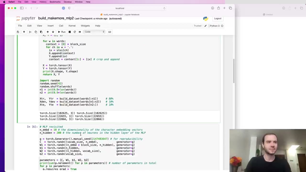 1:53
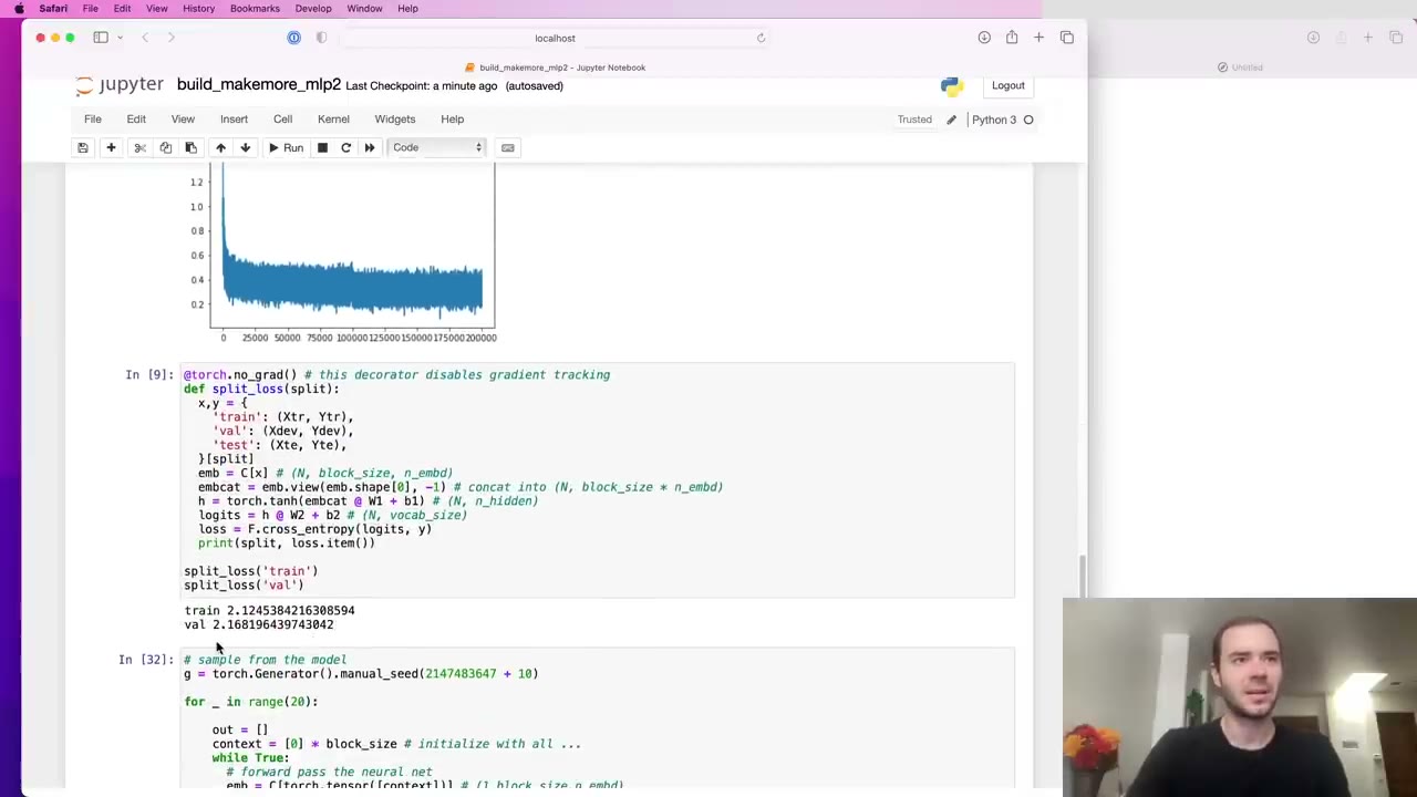 2:37
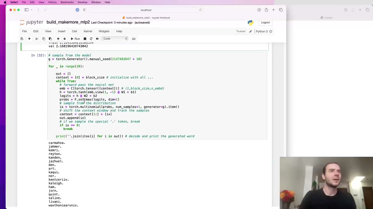 3:52
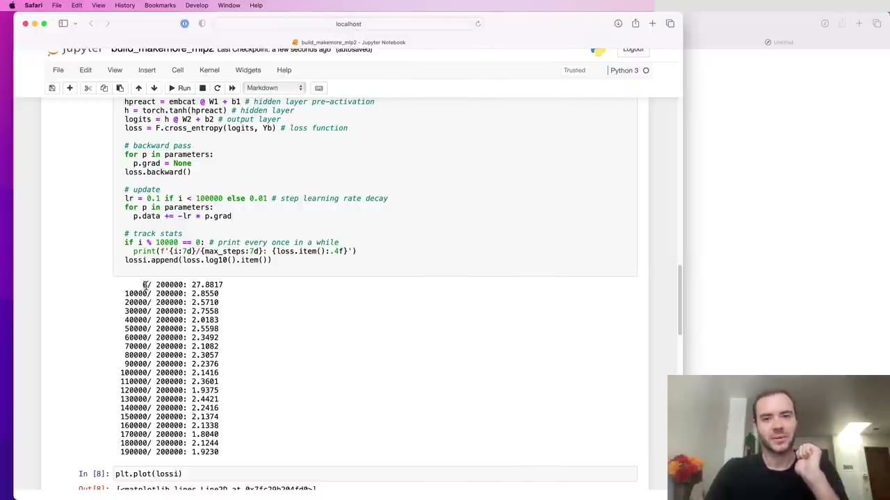 4:32
 6:15
 7:28
 9:09
 11:40
 12:29
 14:45
 15:45
 18:54
 20:38
 25:20
 26:51
 29:07
 30:40
 31:31
 31:44
 32:33
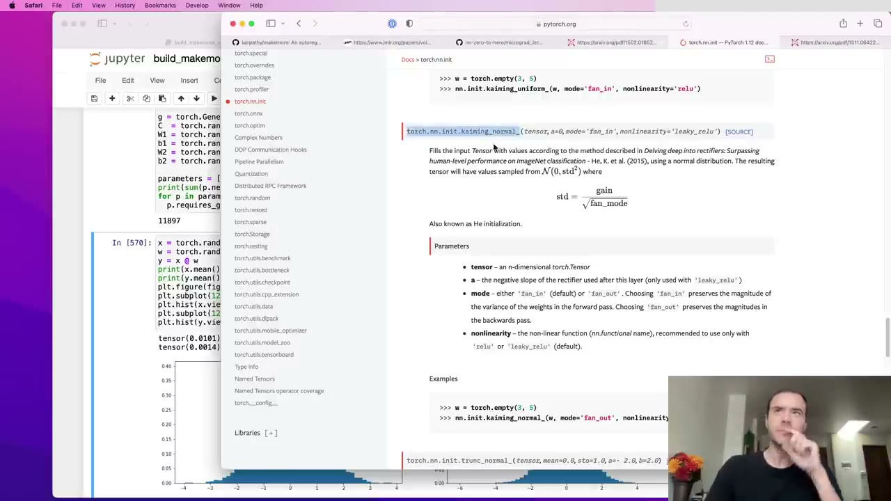 34:07
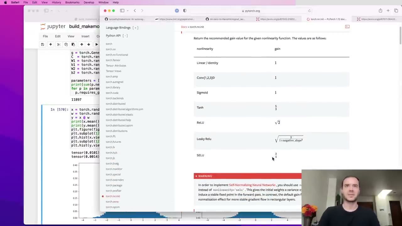 34:51
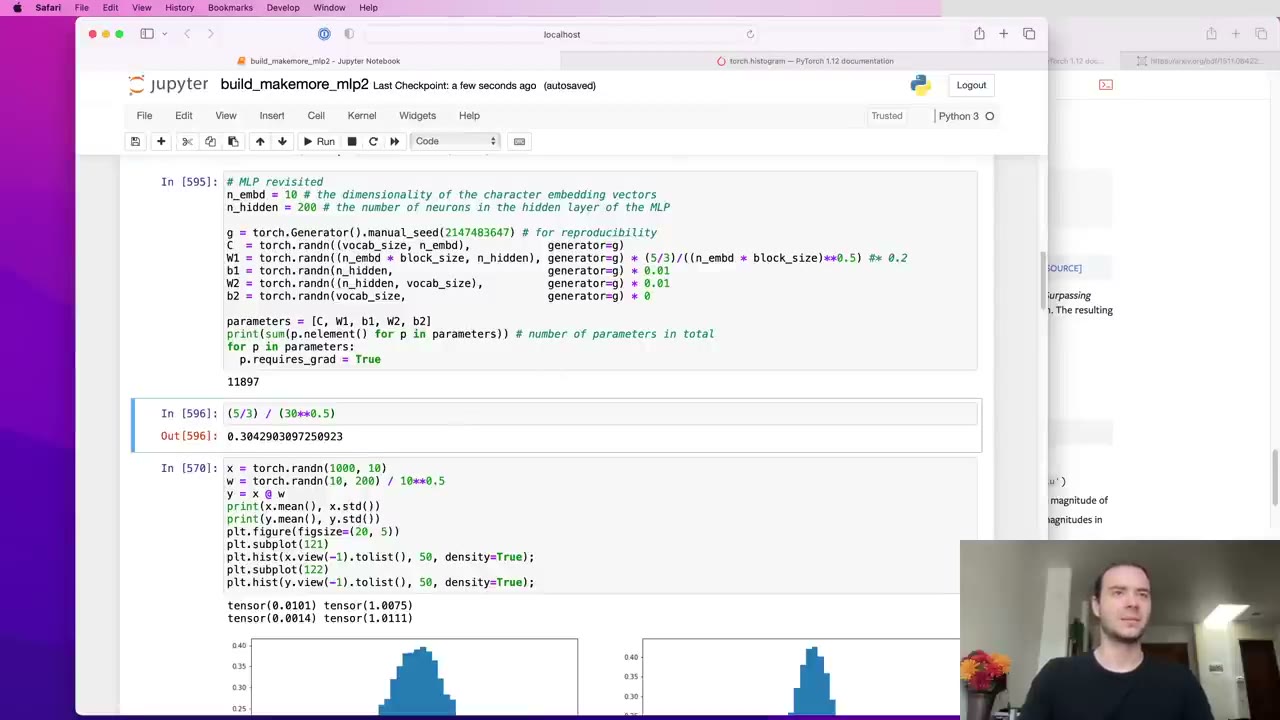 40:02
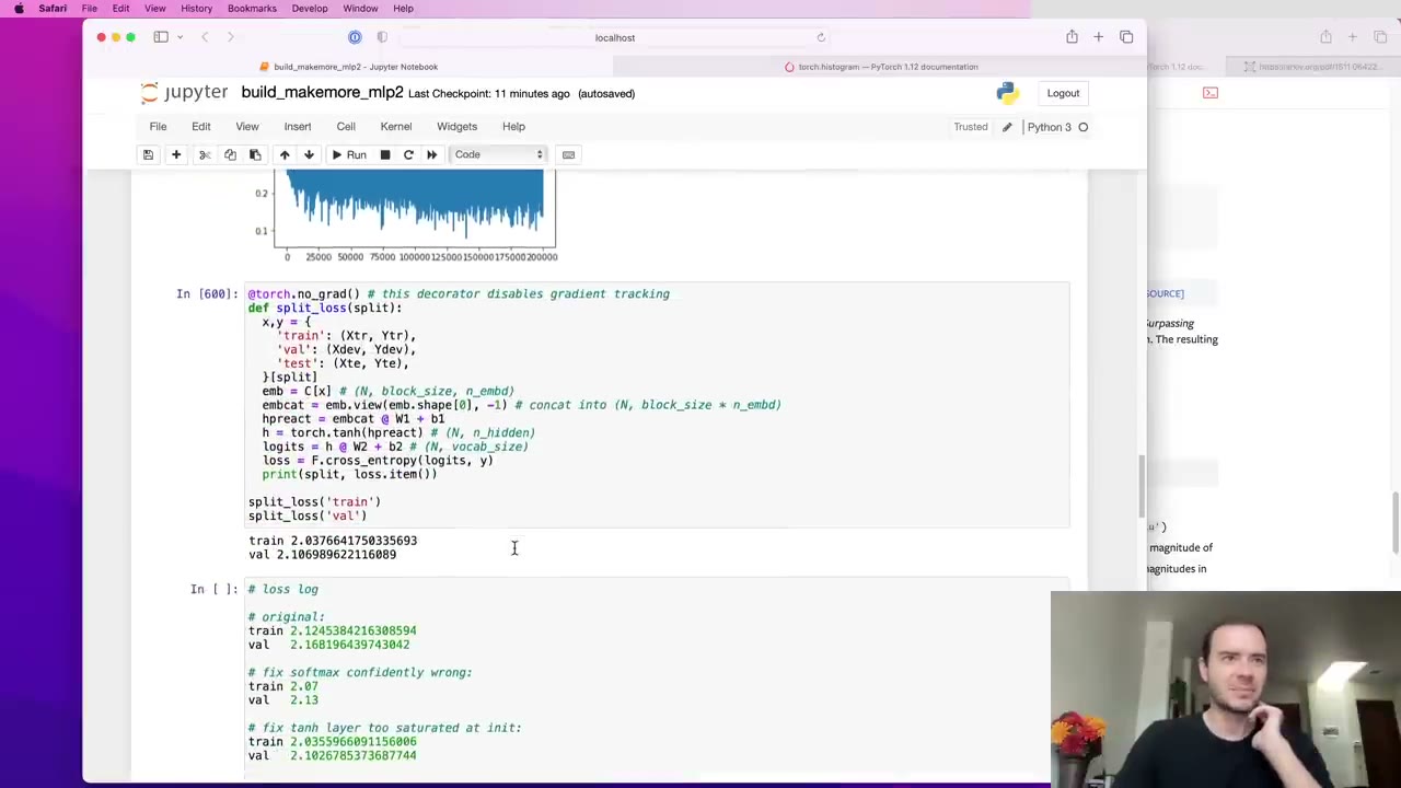 40:10
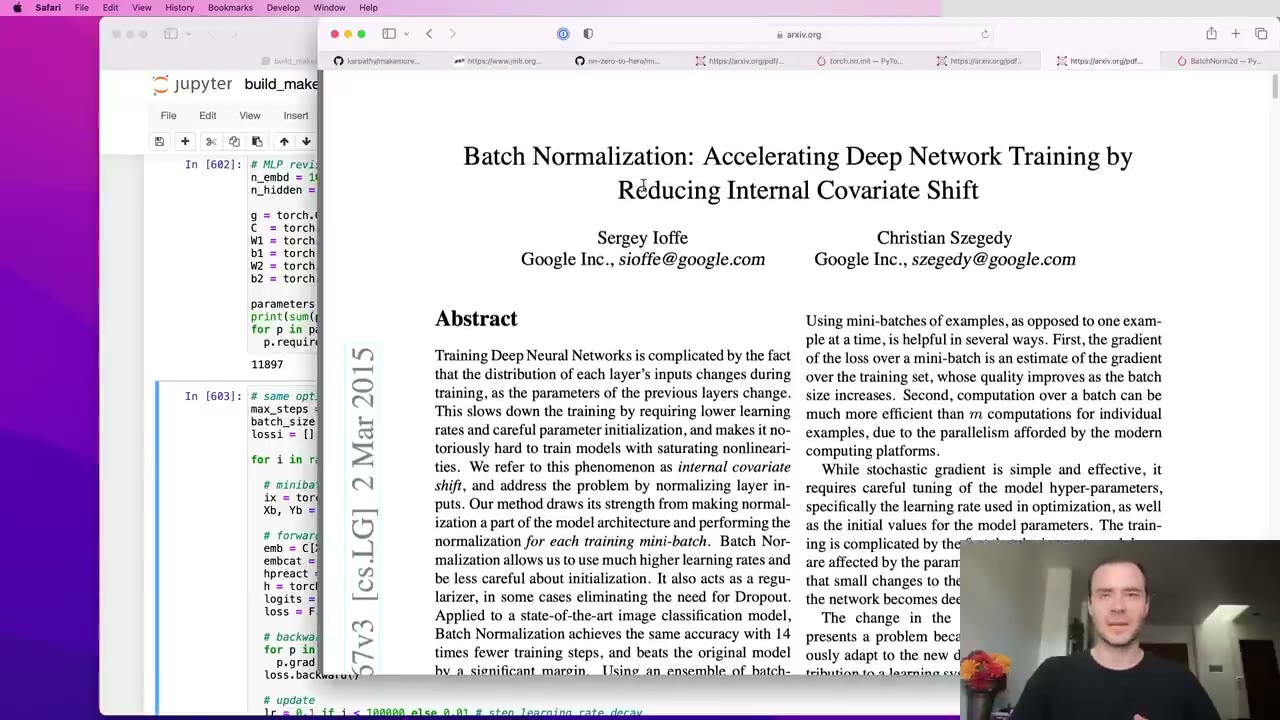 40:51
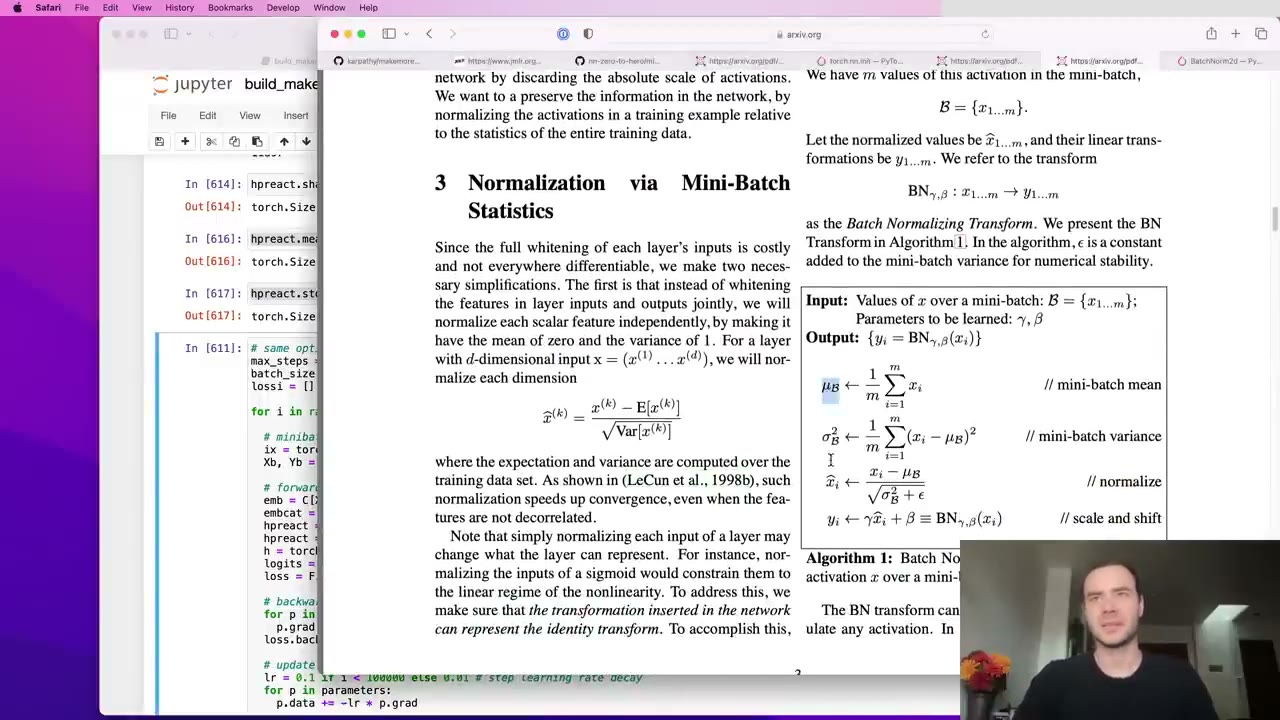 44:42
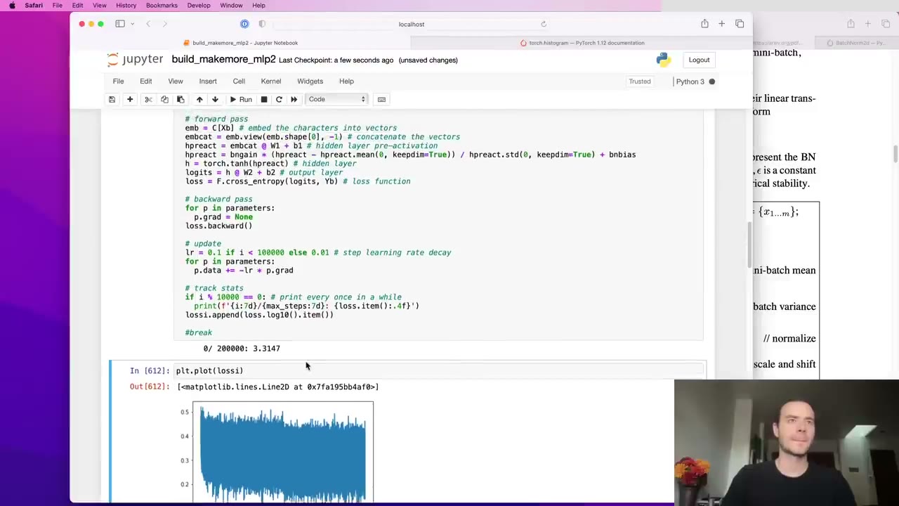 47:42
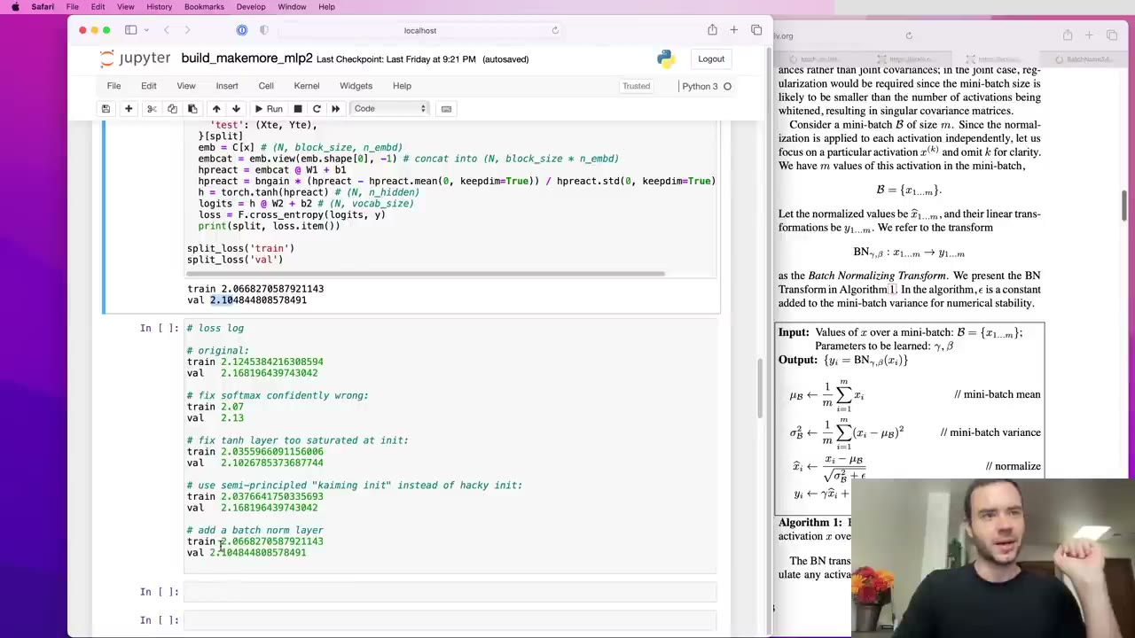 48:25
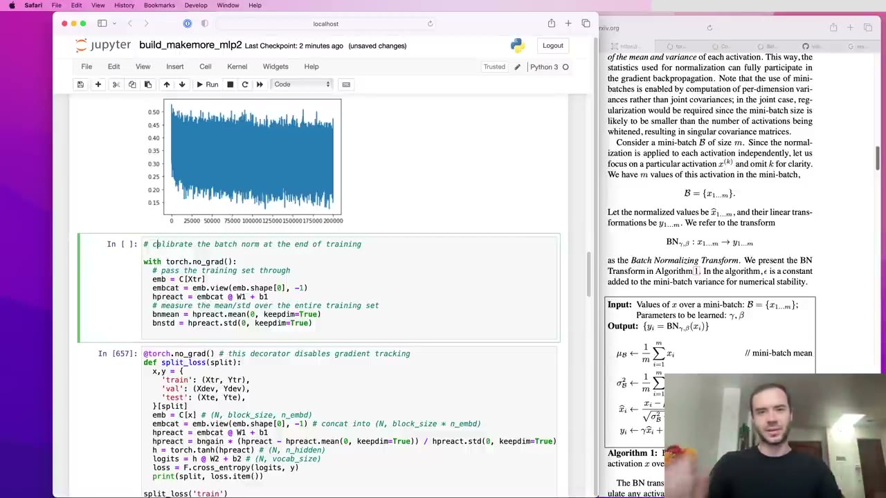 54:57
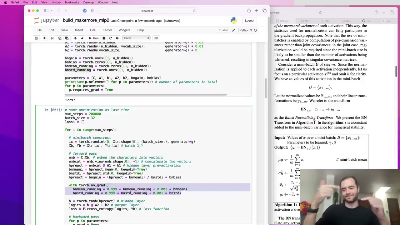 58:48
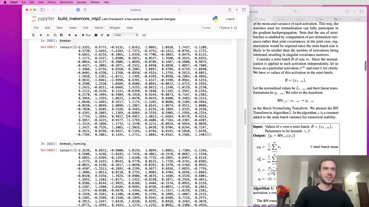 1:00:13
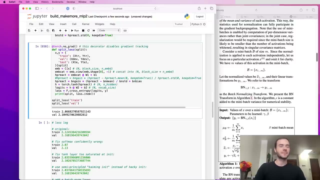 1:00:31
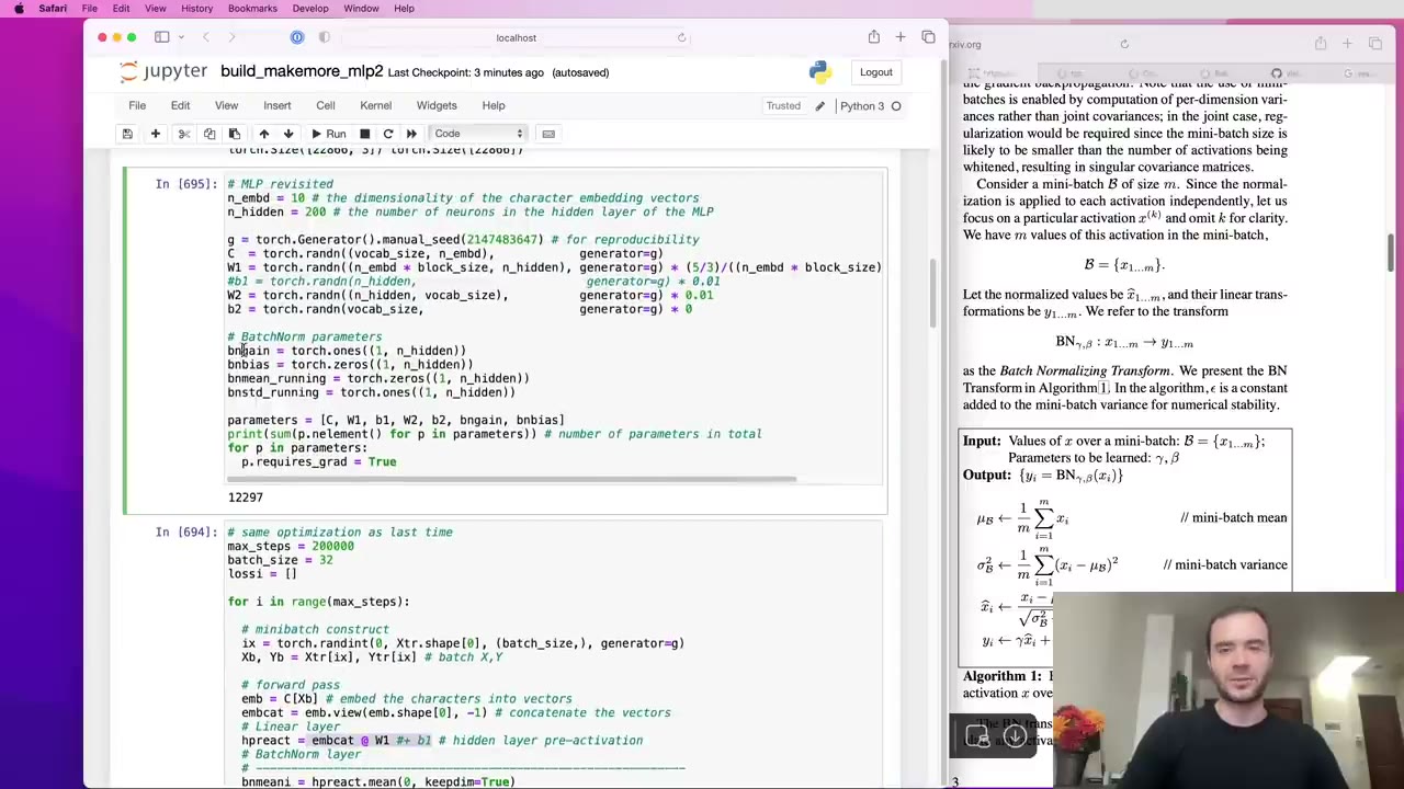 1:03:37
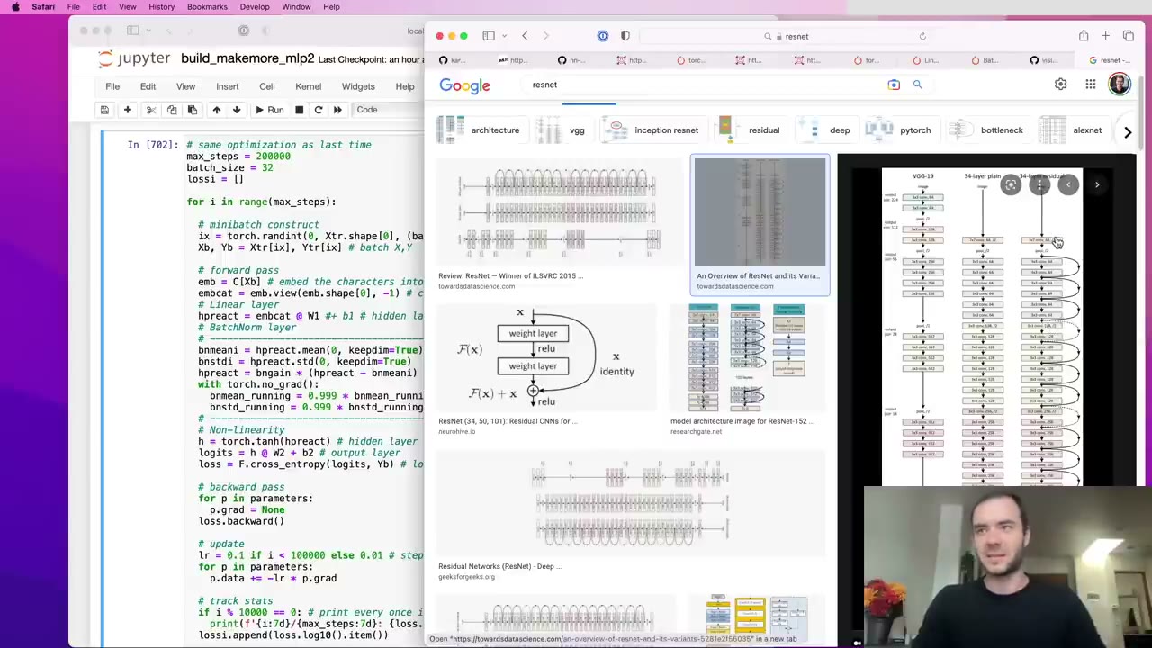 1:05:07
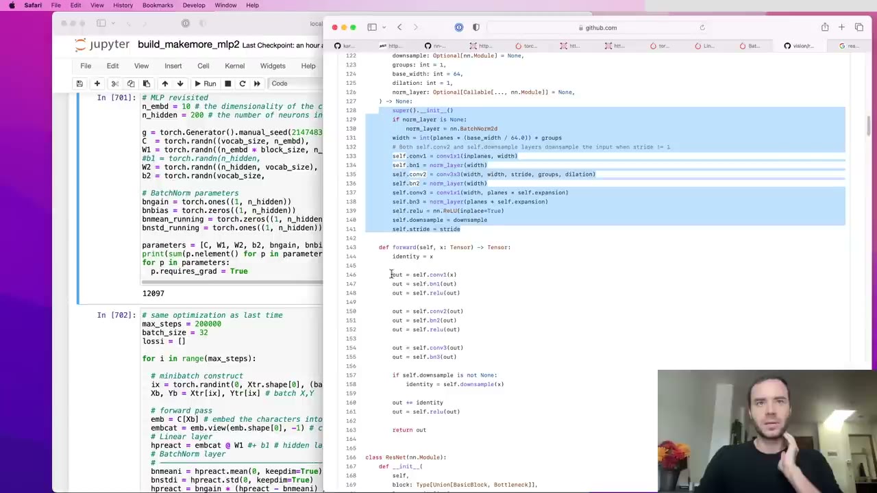 1:05:52
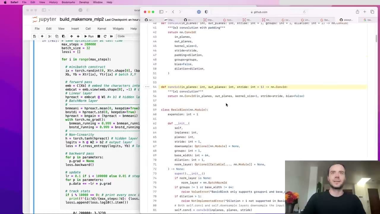 1:07:53
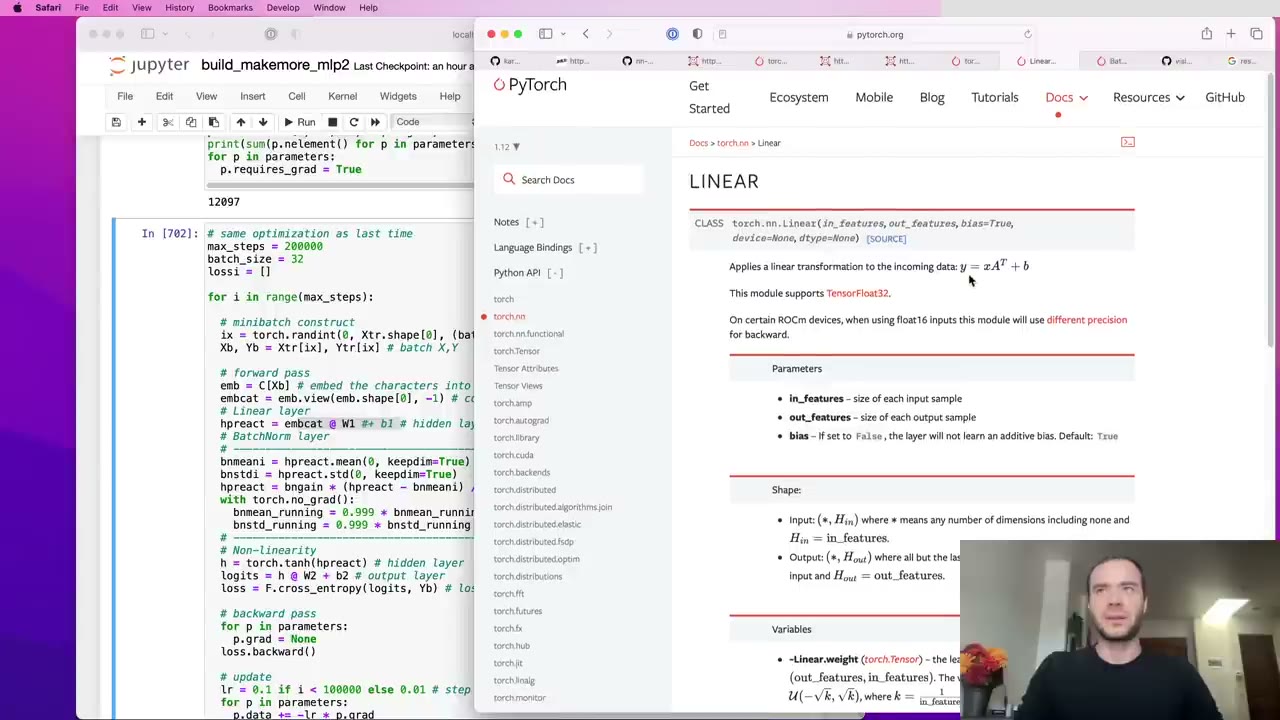 1:09:12
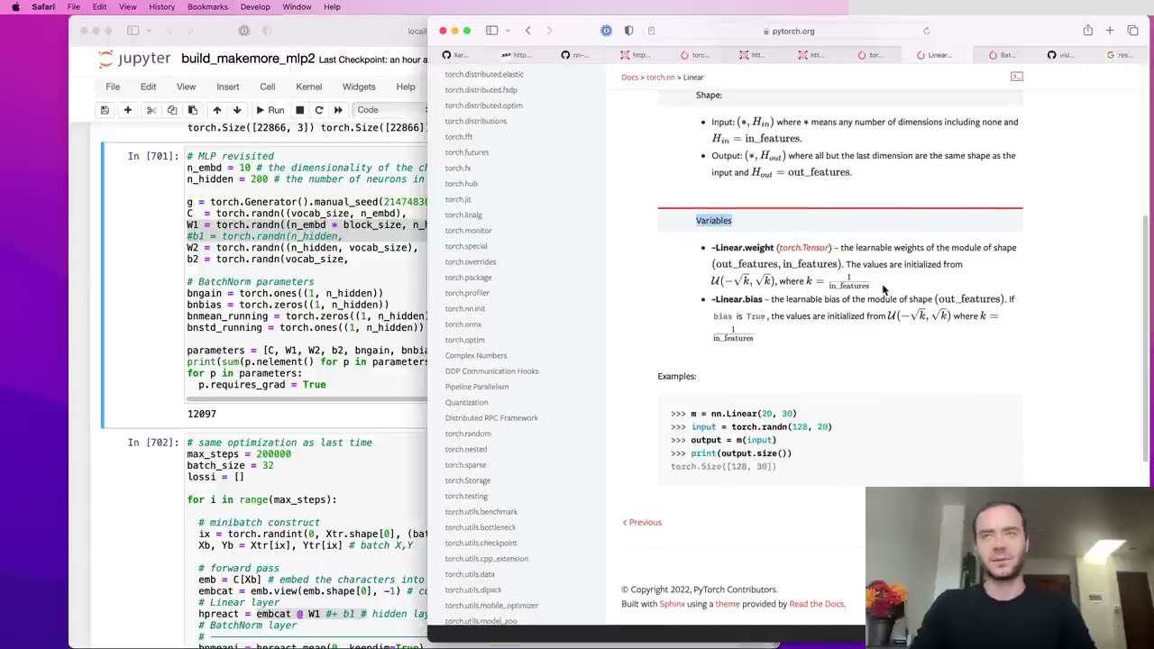 1:10:11
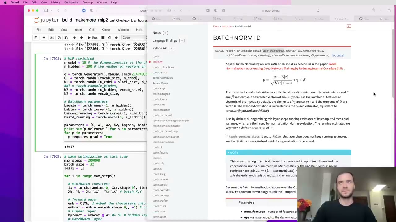 1:11:46
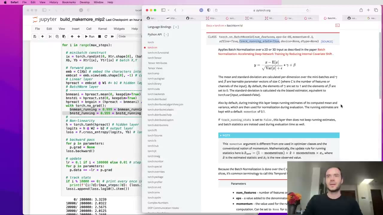 1:13:48
 1:17:19
 1:19:34
 1:24:05
 1:25:21
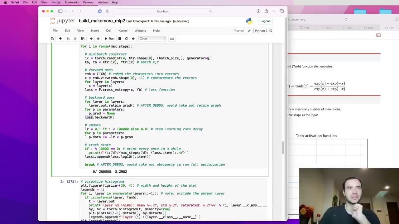 1:26:43
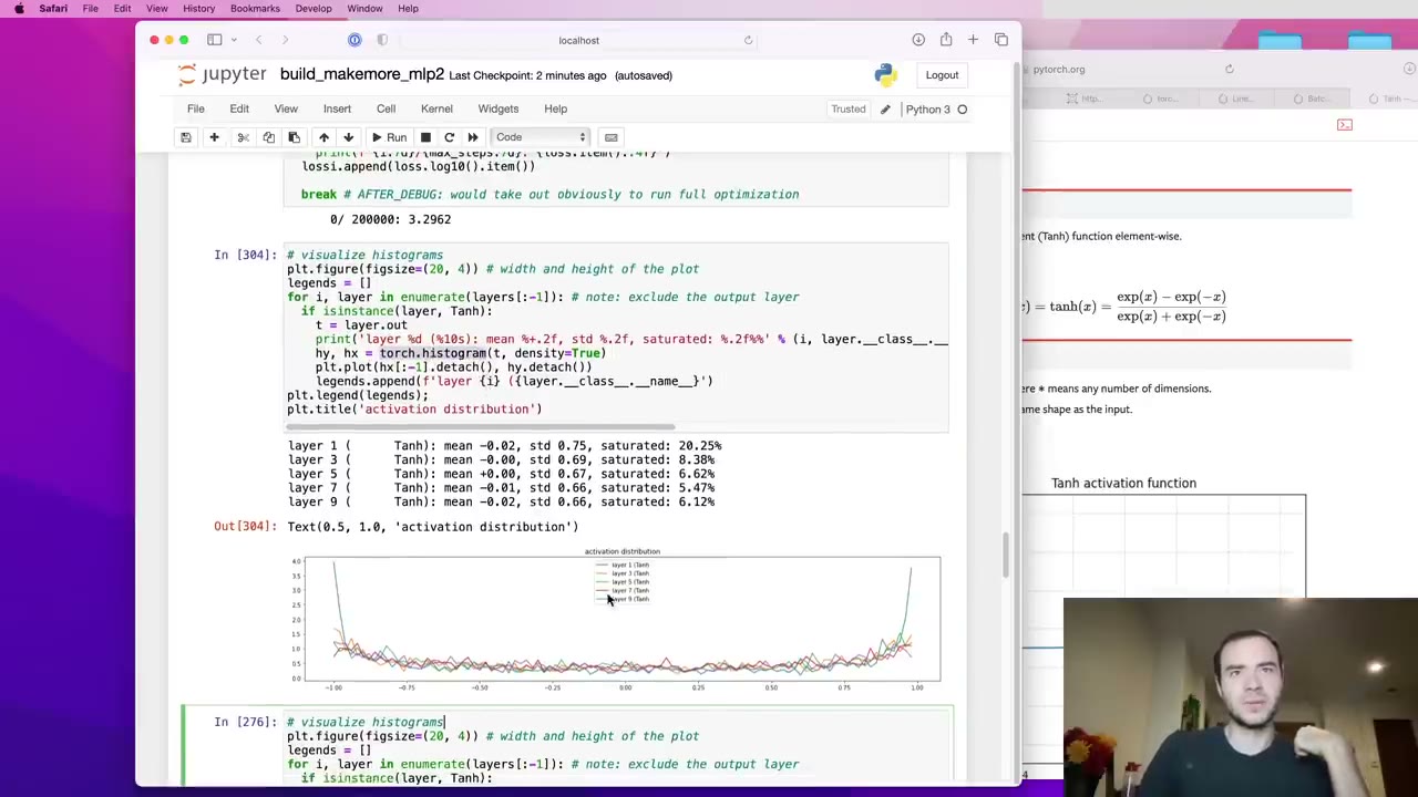 1:27:52
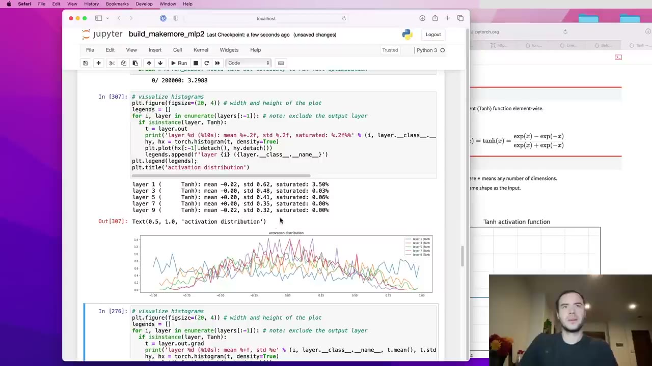 1:28:50
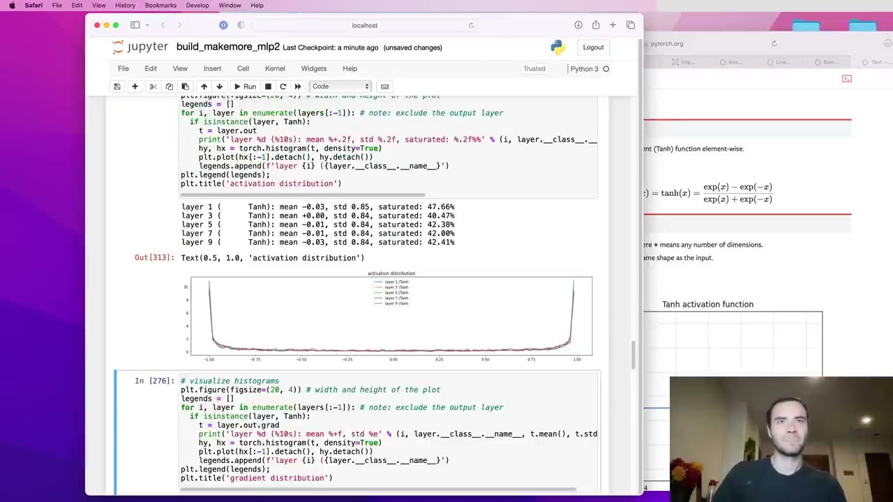 1:30:02
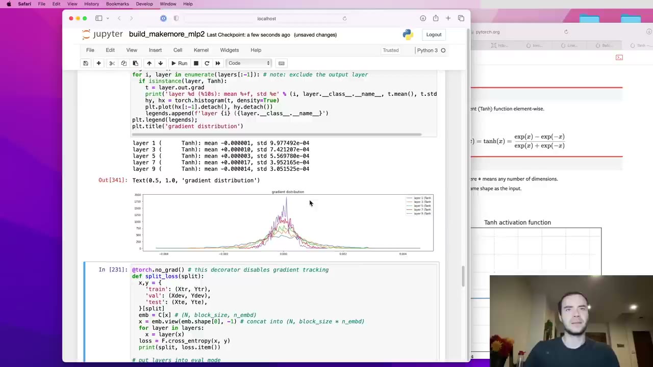 1:31:47
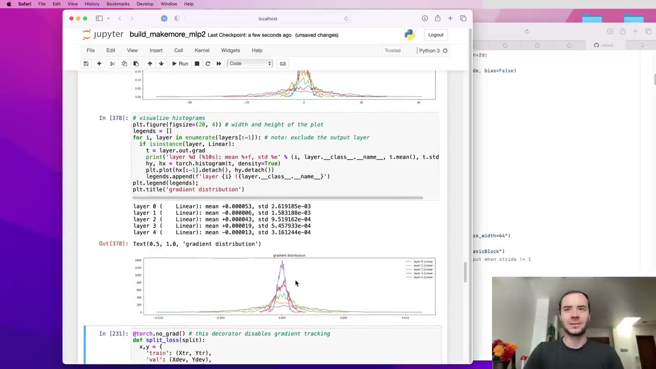 1:32:59
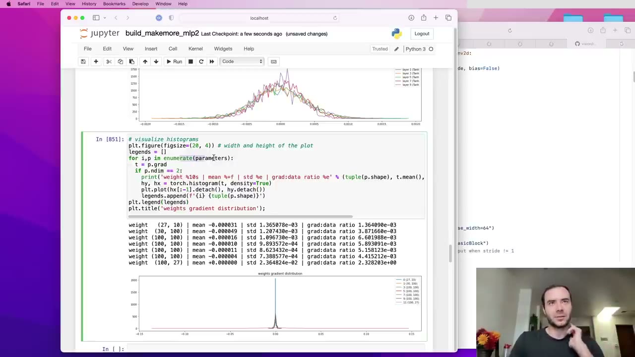 1:36:46
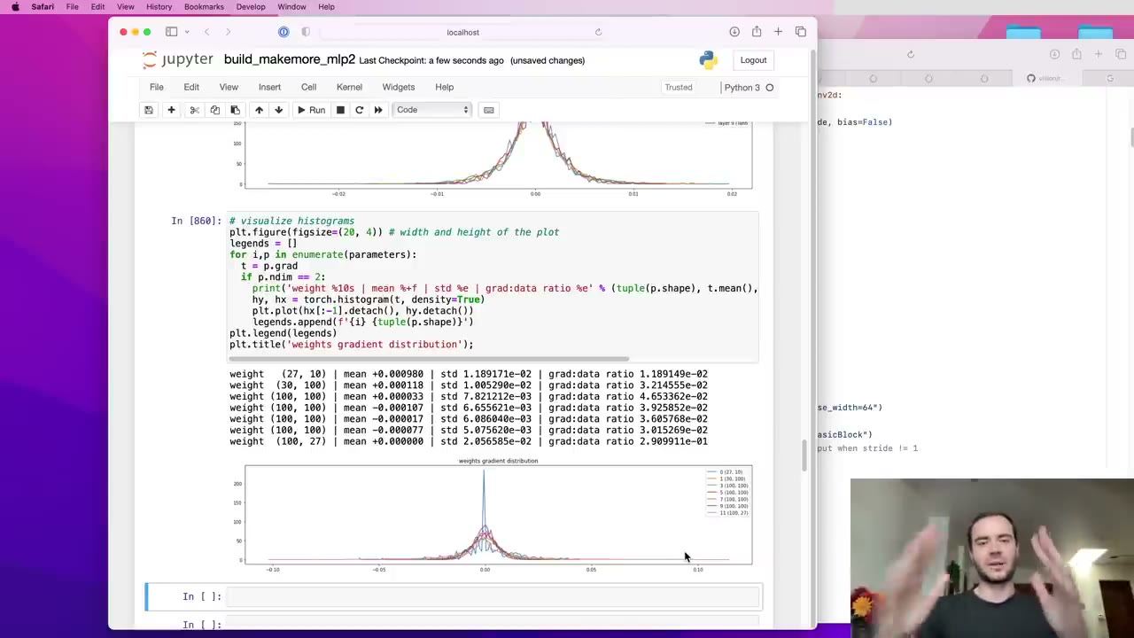 1:39:45
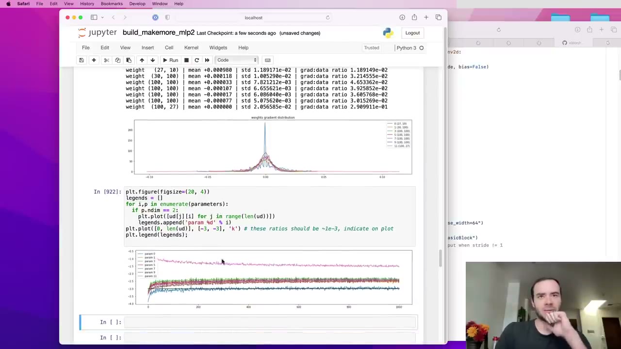 1:41:57
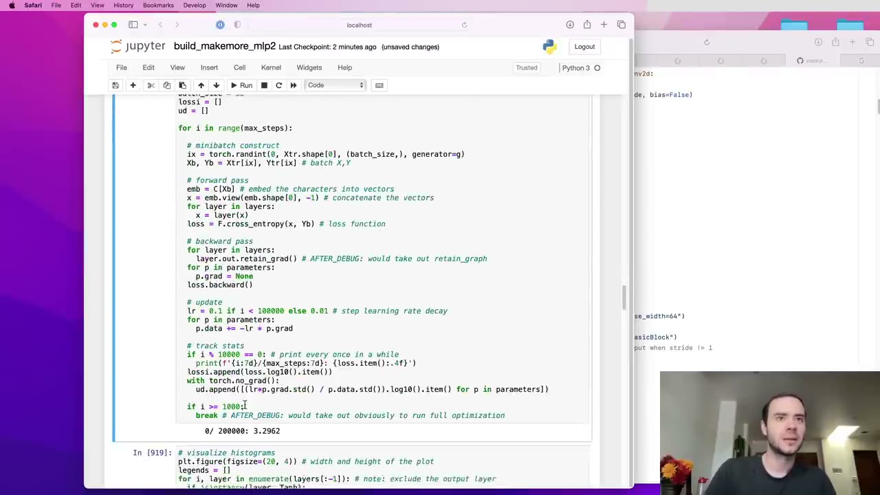 1:43:43
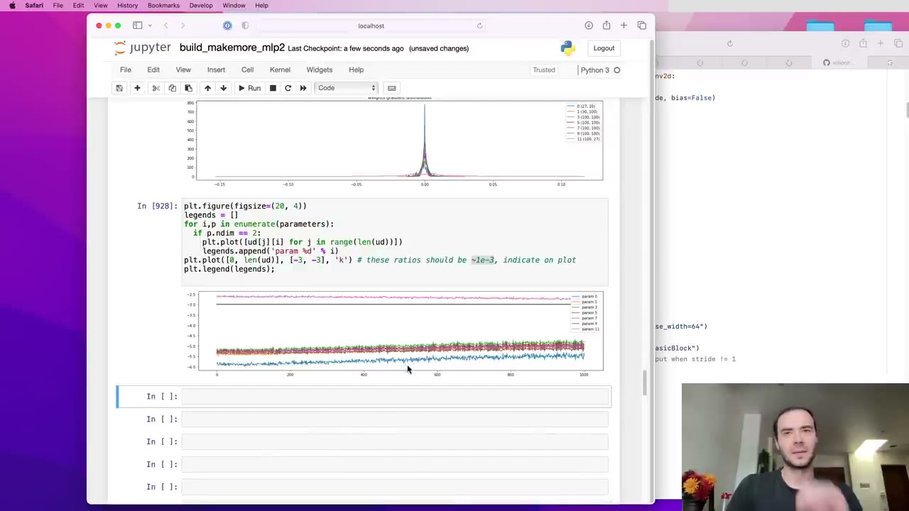 1:43:56
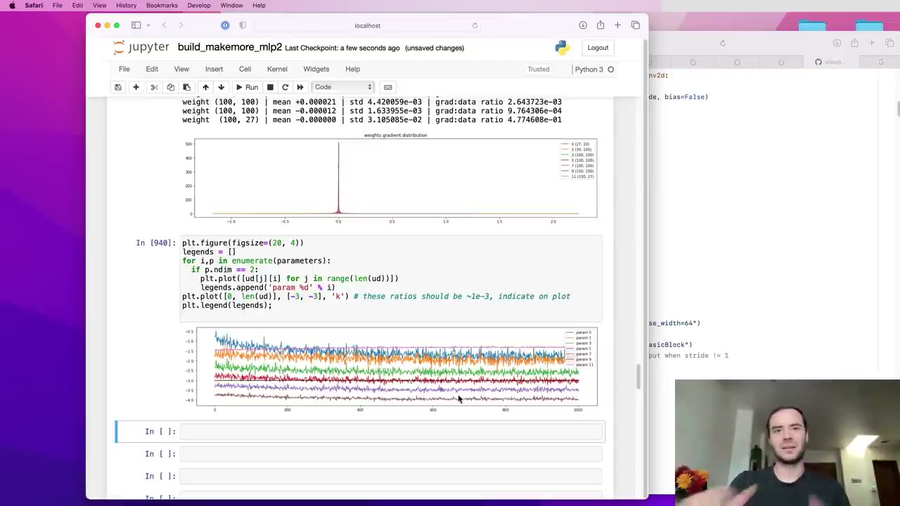 1:45:34
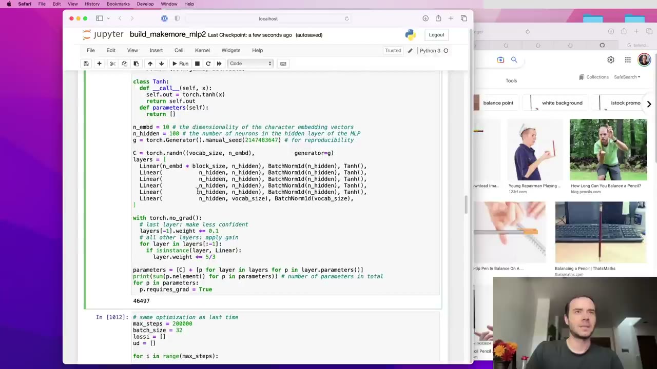 1:47:14
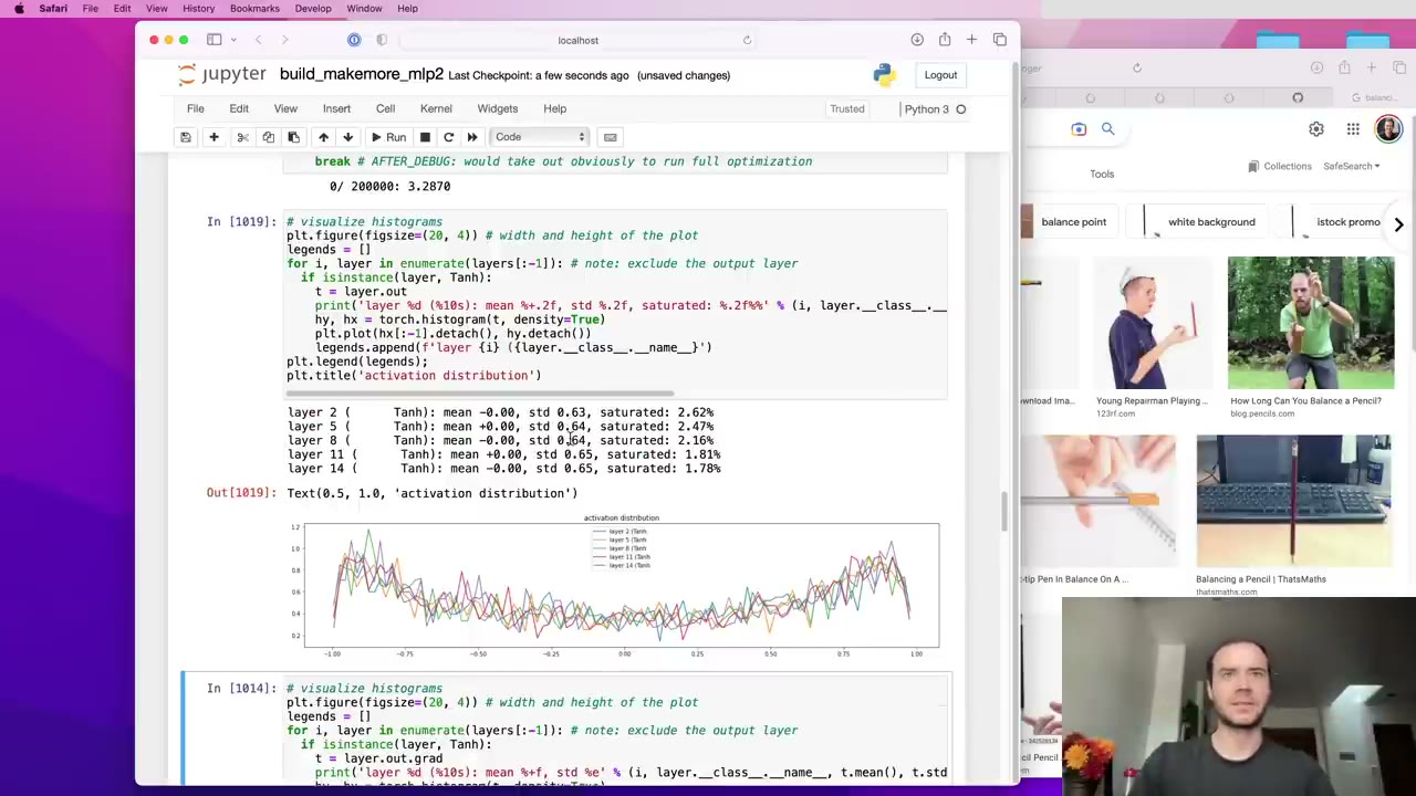 1:47:47
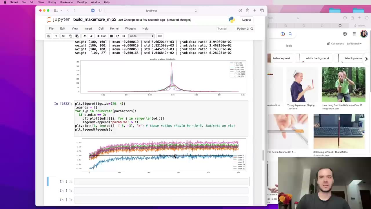 1:48:12
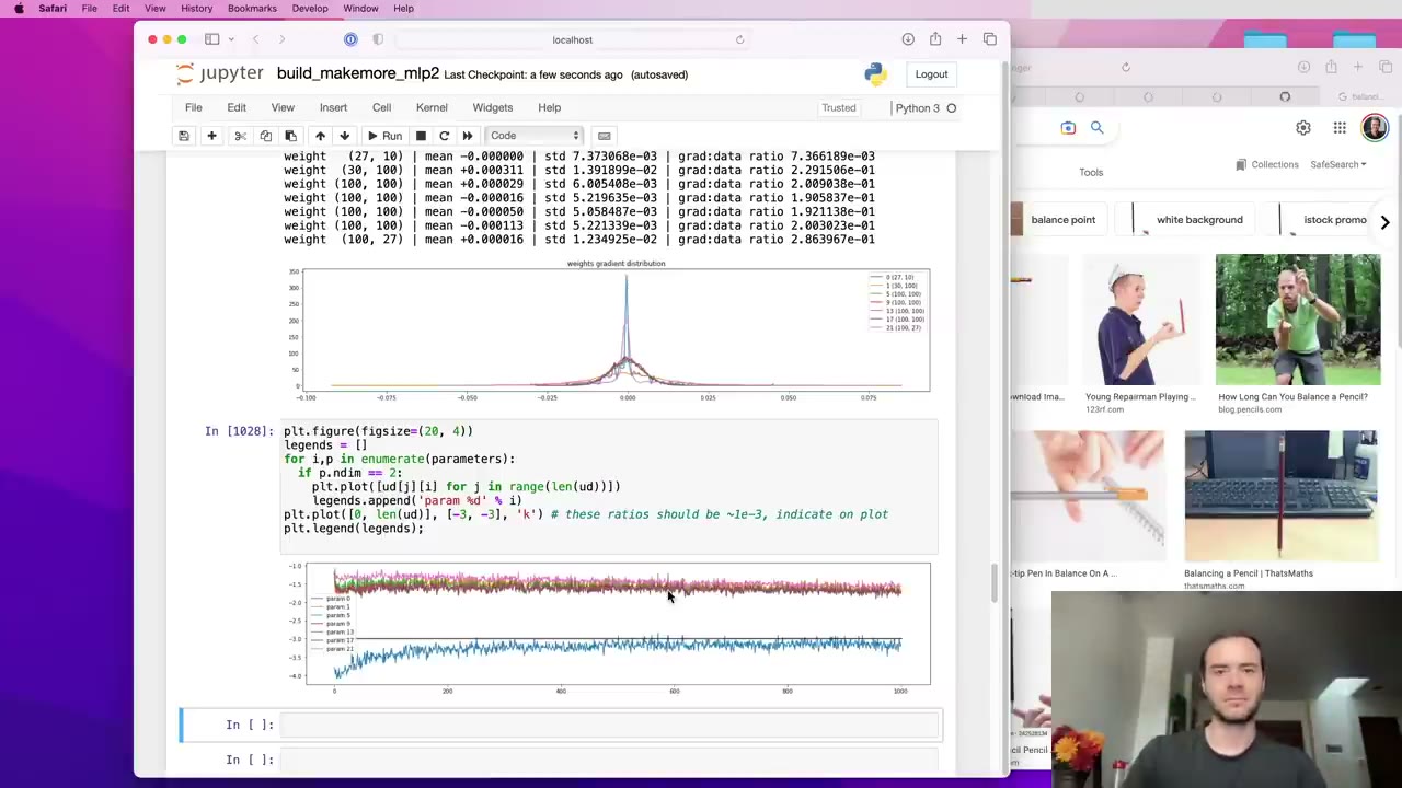 1:49:09
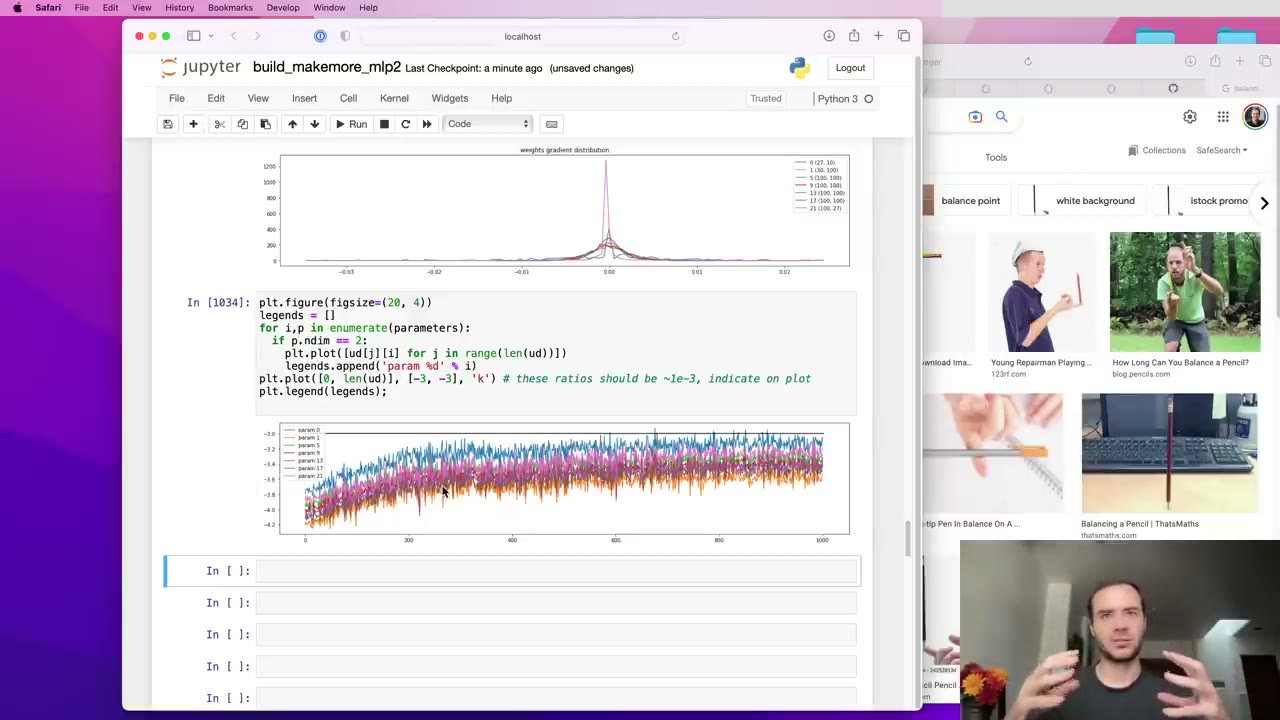 1:49:46
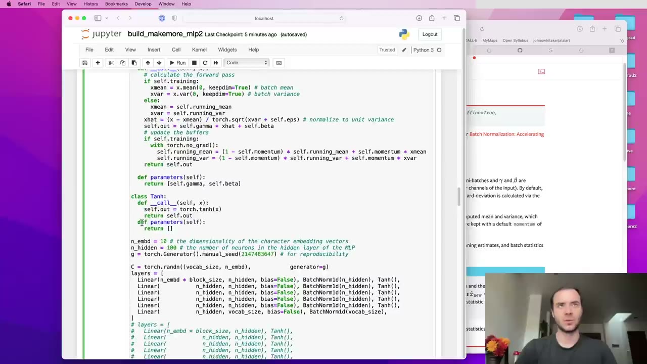 1:52:18
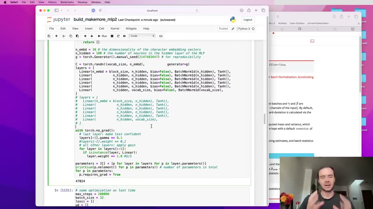 1:54:12
Watch the video (116 min)
Watch the original video on YouTube
Lecture 4 of Andrej Karpathy’s Neural Networks: Zero to Hero pauses the march toward bigger architectures. The character-level MLP from Lecture 3 already trains, but Karpathy wants students to see what goes on inside it: how the activations are distributed in the forward pass, and how the gradients behave on the way back. His reason is historical. Recurrent networks are expressive but hard to optimize, and most later architecture changes were attempts to keep activations and gradients well behaved. The lecture fixes two initialization bugs in the existing model, derives a principled way to scale weights, builds batch normalization from scratch, then rewrites the code as PyTorch-style modules and introduces the diagnostic plots Karpathy uses on his own networks. It is the most practical debugging lecture in the series. The next one, Lecture 5, takes the same network and backpropagates through it entirely by hand.
Key takeaways
- Work out the loss you should see at step zero (5:43). For 27 equally likely characters it is about 3.29. A first loss of 27 means the softmax is confidently wrong, and the first few thousand steps get wasted shrinking the weights.
- Saturated tanh units block the gradient (16:02). The local gradient of tanh is 1 − t², so outputs near ±1 pass almost nothing backward. A unit that sits in the tails for every example is dead and never learns.
- Scale weights by gain / √fan_in (37:22). This keeps activations roughly unit Gaussian from layer to layer. The gain compensates for the squashing nonlinearity: √2 for ReLU, 5/3 for tanh.
- BatchNorm simply standardizes the pre-activations over the batch (44:09), then lets the network rescale and shift them through a learned gain and bias.
- The price is that examples in a batch become coupled (50:21). The resulting jitter acts as a regularizer, but it also causes bugs and forces separate behavior at inference, handled with running statistics.
- Look at the network, not just the loss (1:41:58). Histograms of activations and gradients per layer, plus the update-to-data ratio over time (aim for roughly 1e-3), show miscalibration within a few steps.
- BatchNorm makes a deep net robust to weight scale, not to the learning rate (1:48:44). Forward and backward statistics stay healthy whatever the gain, but the size of the updates changes, so the learning rate may need retuning.
Chapter notes
0:02 – 4:10 Why stay with the MLP, and the starting code
Karpathy explains the detour (0:33). Before moving on to recurrent networks, GRUs and LSTMs, he wants an intuitive feel for activations and gradients during training, because that is what explains why RNNs are hard to optimize with first-order gradient methods and why so many variants were invented.
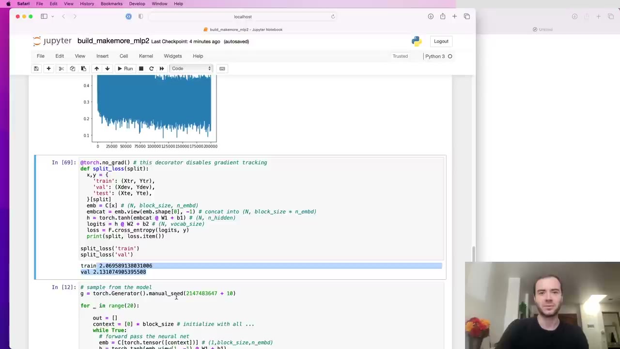
The code is Lecture 3’s MLP with the magic numbers pulled out into named settings (1:34): n_embd for the embedding size and n_hidden for the hidden layer. The network has about 11,000 parameters and trains for 200,000 steps with batches of 32, reaching a train loss of about 2.12 and a validation loss of about 2.17 (2:36). One new tool: the evaluation function is wrapped in @torch.no_grad() (3:06), which tells PyTorch not to record the graph because .backward() will never be called on it.
4:10 – 12:56 Problem one: a loss of 27 at step zero
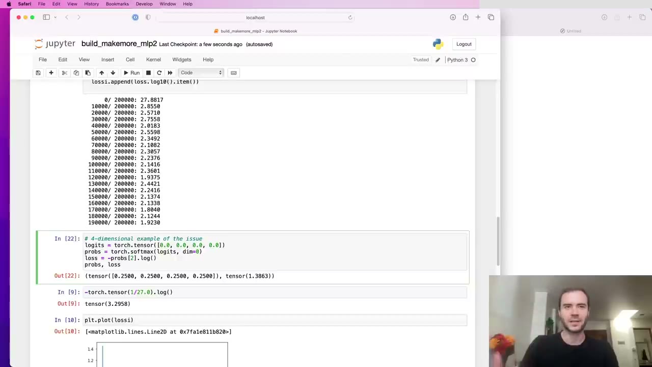
The first logged loss is 27, which then drops fast (4:10). Karpathy’s habit is to predict the initial loss from the setup. With no information, each of 27 characters should get probability 1/27, and the negative log of that is 3.29 (5:43).
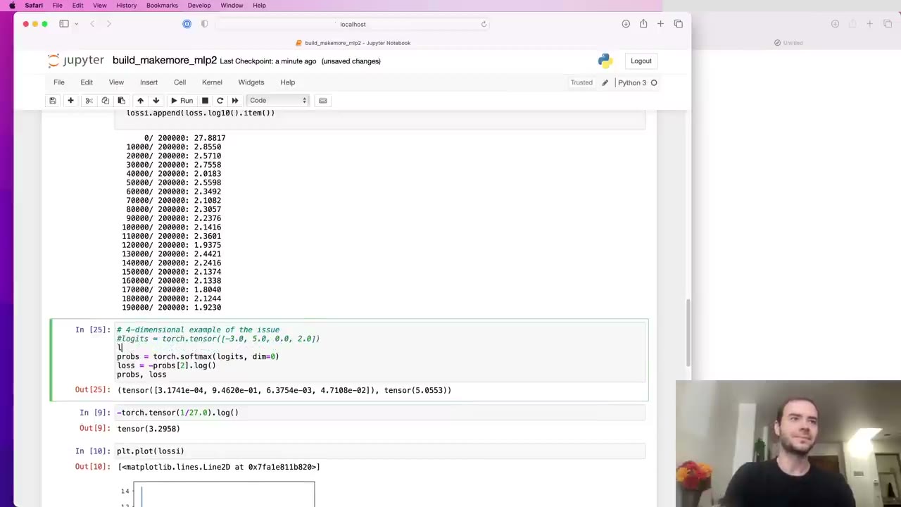
A four-character toy example shows the mechanism (6:13). Logits near zero give a uniform softmax and a loss of 1.38 whatever the label. Scale the logits up and some wrong class almost always wins by a wide margin, so the loss climbs, in the limit to infinity. Logits don’t have to be exactly zero, just equal, but zero is the natural target (8:17).
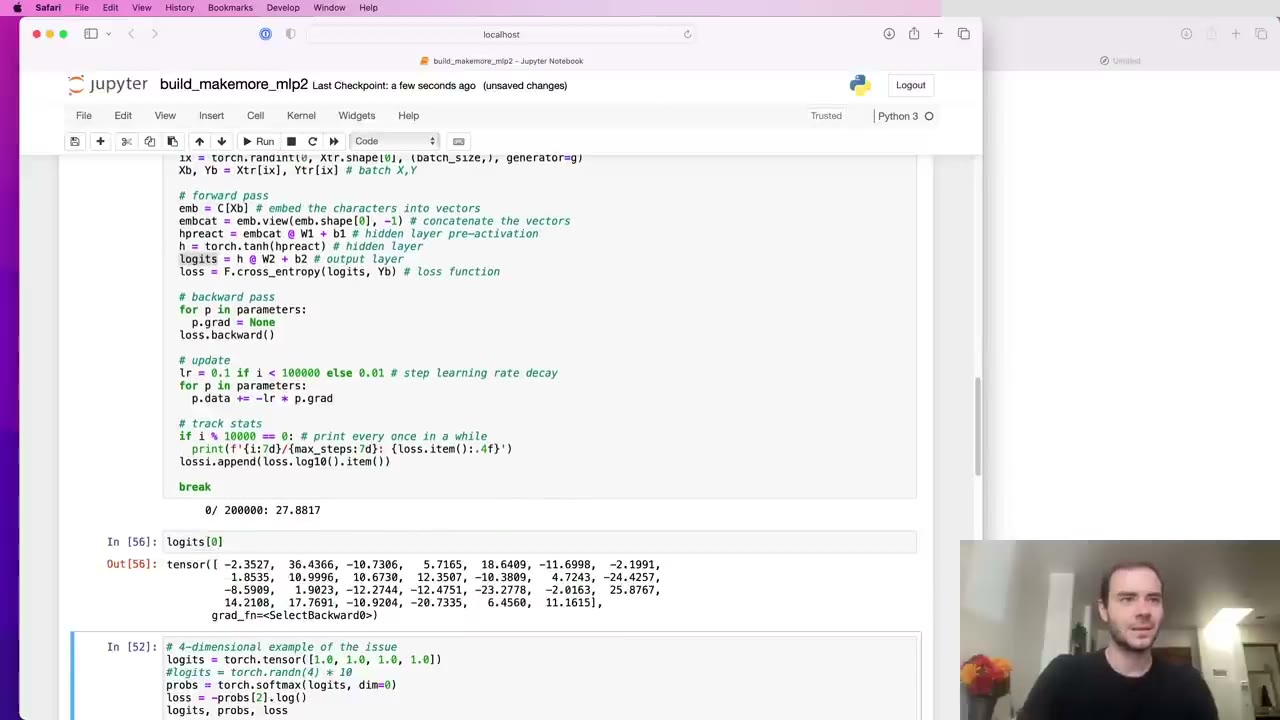
The fix follows from logits = h @ W2 + b2 (9:20): set the output bias to zero and shrink W2. At 0.01 the first loss is close to 3.29. Karpathy avoids exactly zero for weights, keeping a little randomness for symmetry breaking (10:55).
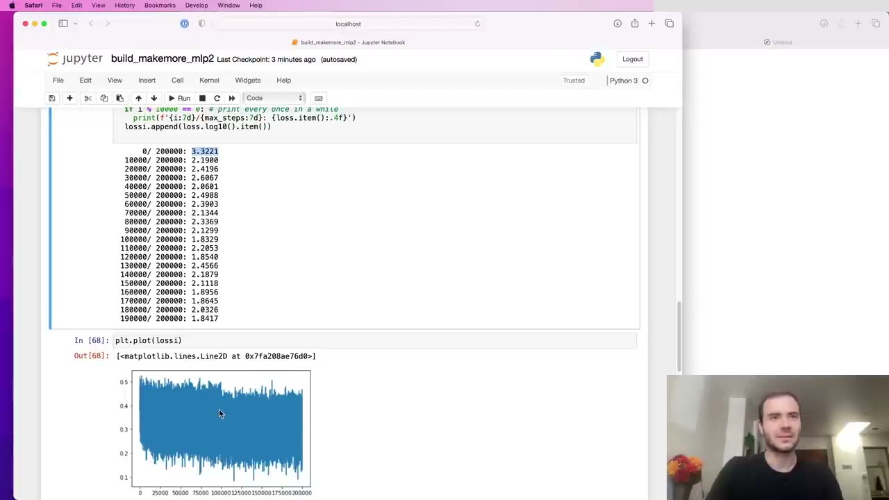
Retrained, the loss curve loses its hockey-stick shape (11:26). That steep early drop was the optimizer doing easy work, squashing oversized logits. With it gone, the steps go into real learning, and the final loss improves slightly (12:26).
12:56 – 23:45 Problem two: a saturated tanh layer, and dead neurons
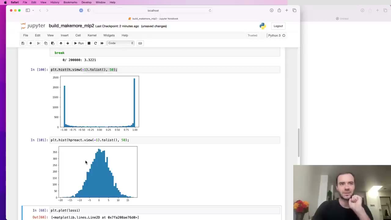
With the logits fixed, the next problem is inside: the hidden activations h (12:56). A histogram shows most values sitting at −1 or 1 (13:57), because the pre-activations range from about −5 to 15 (14:28). Anyone who knows backprop, Karpathy says, is “sweating” at this picture.
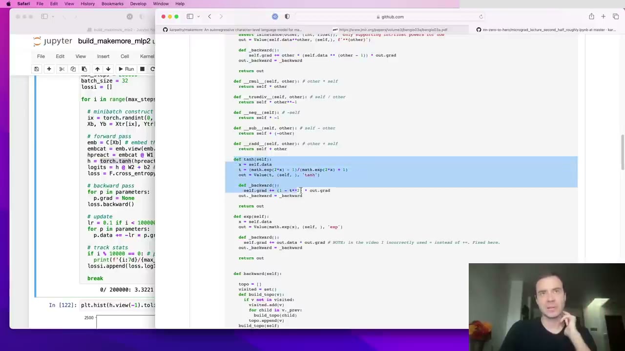
He returns to micrograd’s tanh to explain why (15:30). The backward pass multiplies the incoming gradient by 1 − t². At t = ±1 that is zero and the gradient stops; at t = 0 it passes through unchanged (17:04). The intuition: in the flat tail, nudging the input barely moves the output, so the weights feeding that unit have no influence on the loss. The gradient through tanh can only shrink.
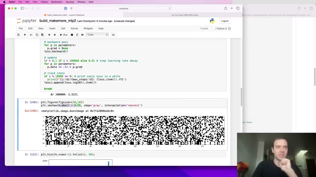
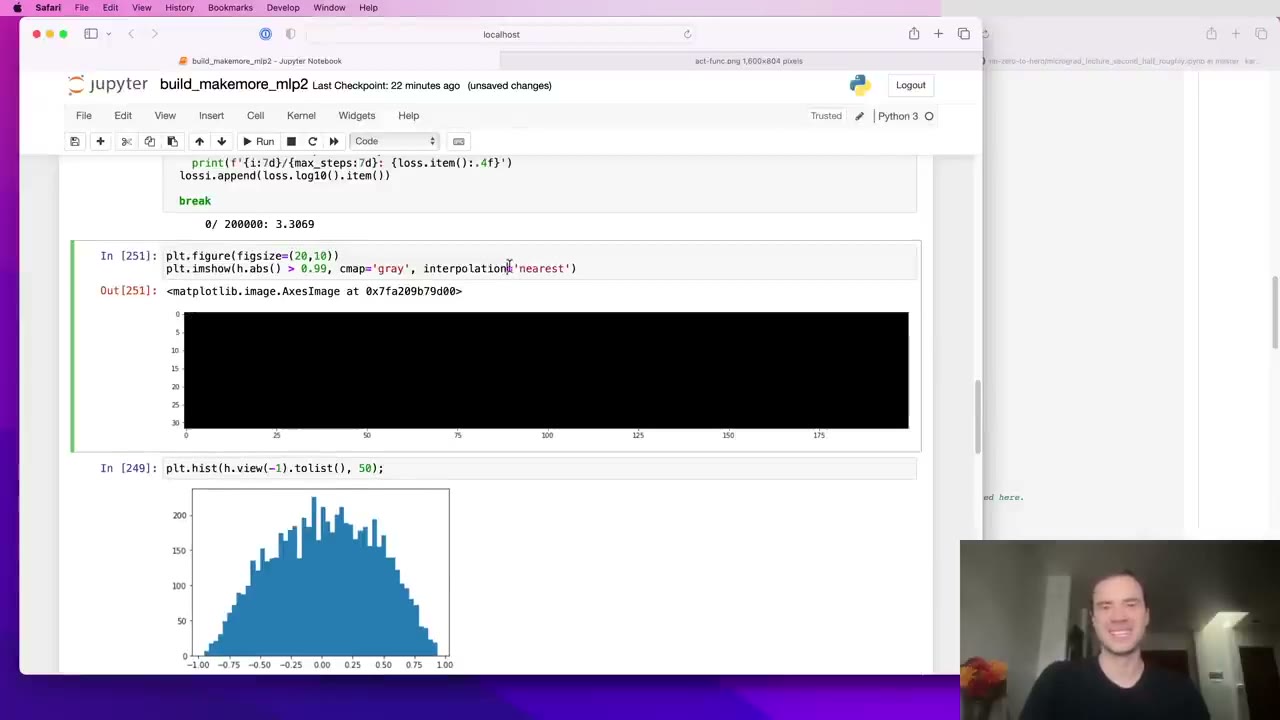
A white-on-black image of h.abs() > 0.99 for 32 examples by 200 neurons makes this visible (18:36). The real danger would be a fully white column, a dead neuron that saturates for every input and therefore never learns (19:09). There is no such column here, so the network still trains.
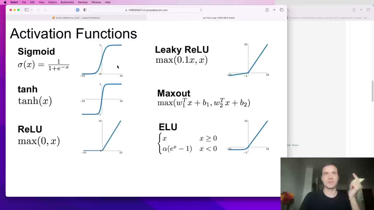
The same failure applies to other activations (20:41). Sigmoid squashes the same way. ReLU is exactly flat below zero, so a ReLU unit that never turns on gets exactly zero gradient. That can happen at initialization by bad luck, or during training when a high learning rate knocks a neuron off the data manifold, which Karpathy calls “permanent brain damage” (22:11). Leaky ReLU avoids flat tails; ELU still has a flat part (22:43).
Our note: a quick audit for your own model is to push the whole training set through and count units that never activate. That is the check Karpathy describes in words at 22:11.
23:45 – 28:05 Fixing the hidden layer, and why shallow nets forgive you
The fix mirrors the logits fix (23:45): bring the pre-activations closer to zero. Biases get multiplied by 0.01 for a little diversity (24:18), weights by 0.1 and then 0.2 by eye, until the histogram looks healthy and no unit exceeds 0.99 (24:50).
The scoreboard after full training (25:55):
| Change | Validation loss |
|---|---|
| Original initialization | 2.17 |
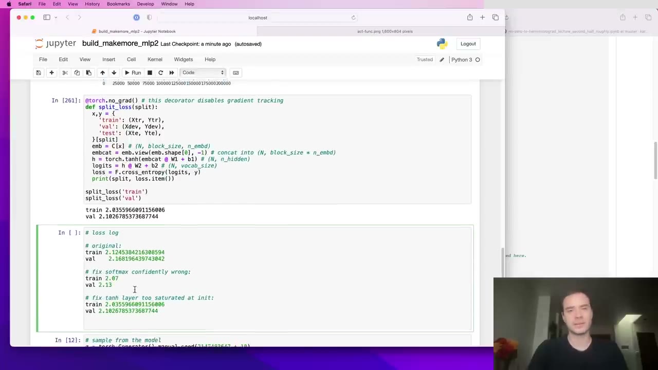
| Fix the overconfident softmax | 2.13 |
| Fix the saturated tanh layer | 2.10 |
Karpathy stresses that a one-hidden-layer MLP is forgiving (27:01). Bad initialization only cost a little here. In a 50-layer network the same mistakes stack up and training can stall completely.
28:05 – 33:48 Preserving a unit Gaussian: divide by √fan_in
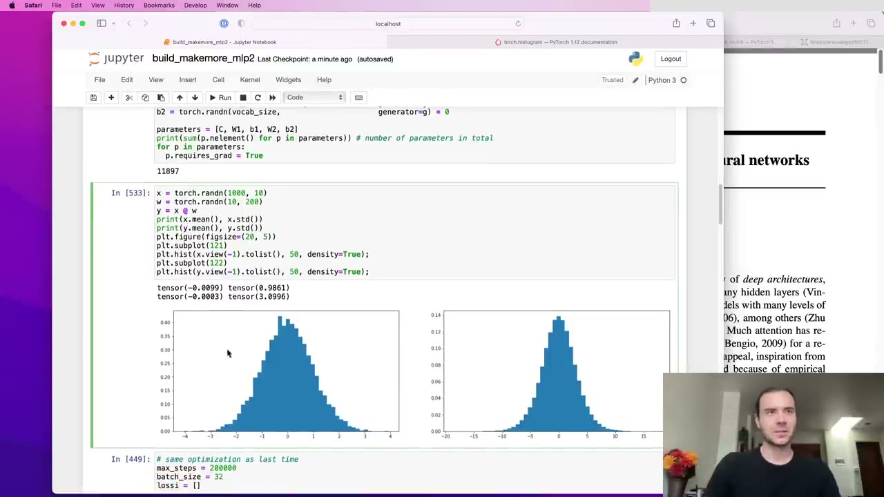
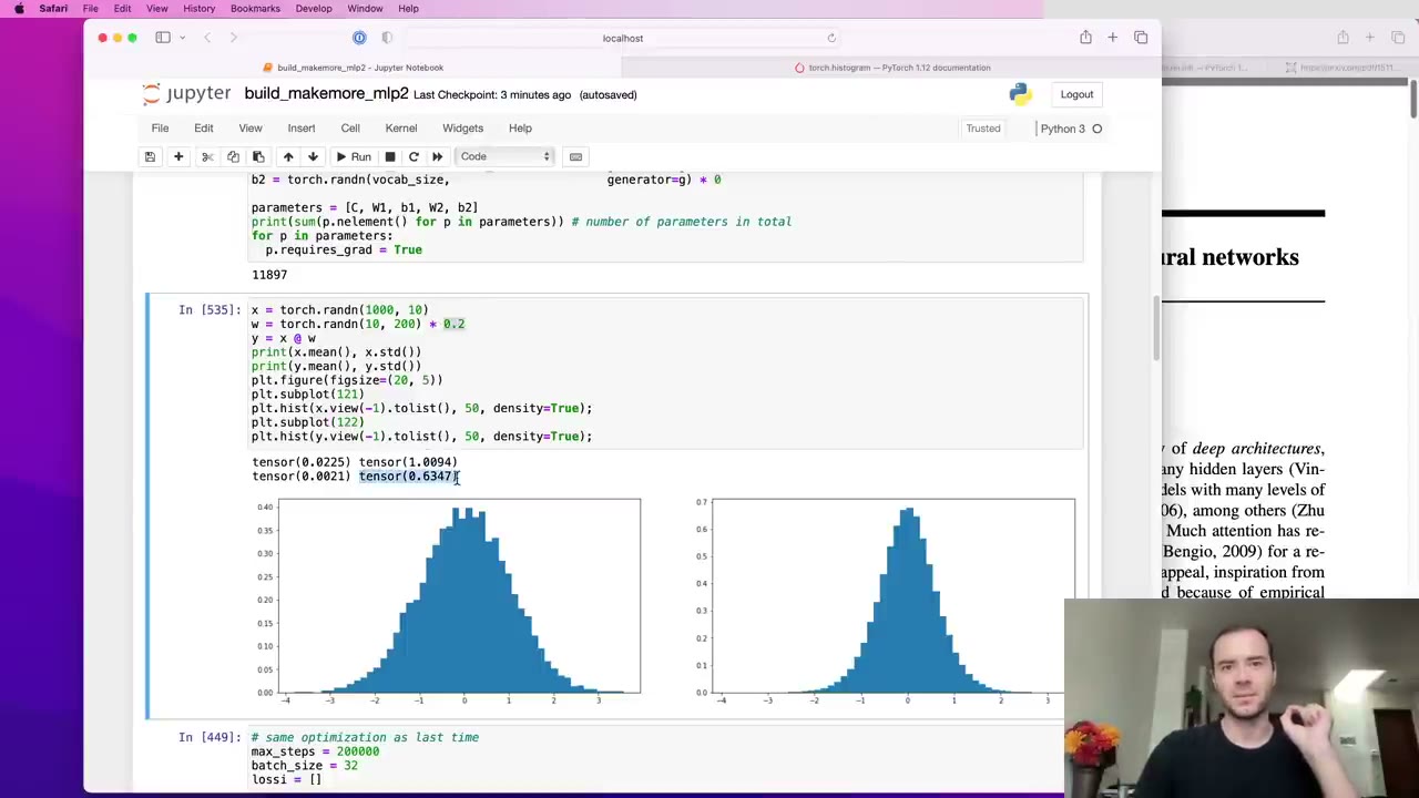
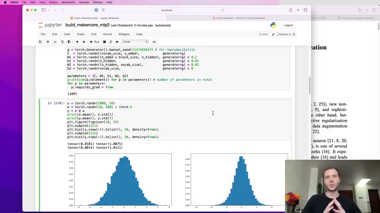
Hand-tuned numbers like 0.2 don’t scale to big networks, so he looks for a rule (28:05). Experiment: 1,000 Gaussian inputs of dimension 10, times a Gaussian weight matrix with 200 outputs. The output’s standard deviation grows from 1 to about 3 (29:07). Scale the weights by 5 and it grows to 15; by 0.2 and it shrinks to 0.6. The variance math says to divide the weights by √fan_in, here √10, and the output comes out at exactly unit standard deviation (30:39).
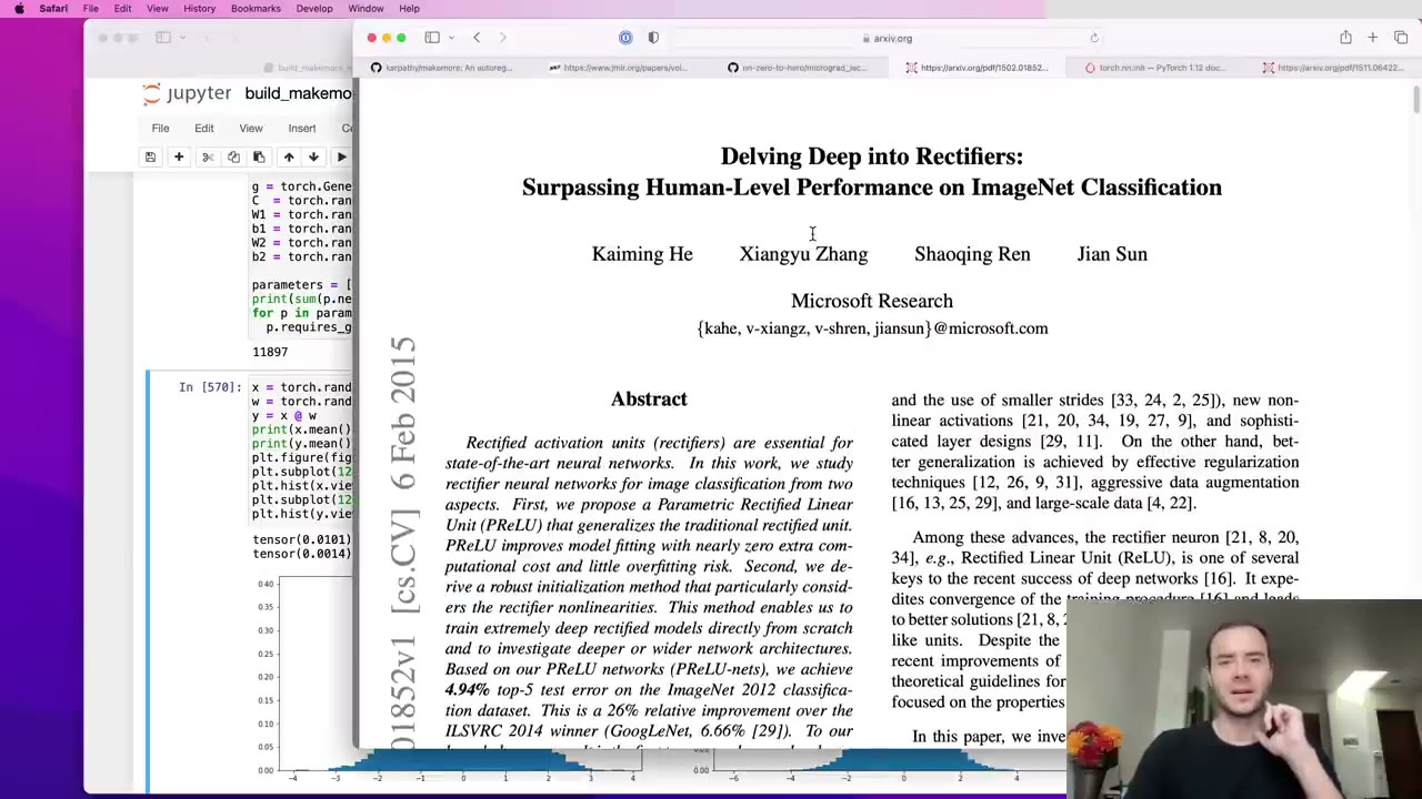
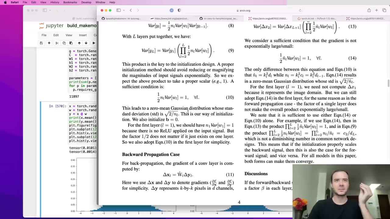
The reference paper is Kaiming He and colleagues’ “Delving Deep into Rectifiers” (31:43), which studies convolutional nets with ReLU and PReLU. Because ReLU discards half of its input distribution, they need an extra factor: weights with standard deviation √(2 / fan_in) (32:14). The paper also analyzes the backward pass and finds that getting the forward pass right gets the gradients roughly right, up to a factor that, empirically, doesn’t matter much (33:16).
33:48 – 40:31 Kaiming init in practice
PyTorch implements this as torch.nn.init.kaiming_normal_ (33:48), which Karpathy calls probably the most common way to initialize networks. Its mode chooses whether to preserve activations (fan_in, the usual default) or gradients (fan_out); its nonlinearity argument sets the gain. For linear it is 1, for ReLU √2, and for tanh 5/3 (34:48). The gain exists because tanh, like ReLU, is contractive: it squeezes the tails, so the weights need a boost to restore unit spread (35:19).
He admits he is moving quickly on purpose (35:49). Around the time of that paper, deep nets were fragile and gains had to be set precisely. Three later innovations made this far less critical: residual connections, normalization layers (batch, layer, group) and better optimizers such as RMSprop and Adam (36:20). His own practice is simply to divide weights by √fan_in.
Applied to the MLP: the fan-in is not 10 but n_embd * block_size = 30, three 10-dimensional characters concatenated (38:58). (5/3) / √30 is about 0.3, close to the hand-tuned 0.2. Training reaches 2.10 again (40:00), the same result without a magic number.
40:31 – 47:48 BatchNorm: just standardize the activations
Batch normalization came out of Google in 2015 and made very deep networks reliably trainable (40:31). The insight Karpathy says blew his mind (41:34): if you want the pre-activations to be unit Gaussian, normalize them. Mean and standard deviation are differentiable, so the whole operation can sit inside the network and be trained through.
Implementation (42:36): hpreact is 32 × 200, so take the mean and standard deviation along dimension 0 with keepdim=True, giving 1 × 200 statistics, then subtract and divide. Each neuron is now exactly unit Gaussian over this batch, hence the name.
Forcing that at every step would hurt, though (45:10). The network should stay free to make a unit fire more readily or more sparingly. So the paper adds a scale and shift: a gain initialized to ones and a bias initialized to zeros, both learned by backprop (45:42). At initialization the output is exactly standardized; after that the network decides.
Our note: the paper is Sergey Ioffe and Christian Szegedy, “Batch Normalization: Accelerating Deep Network Training by Reducing Internal Covariate Shift” (2015). Its γ and β are the bngain and bnbias here.
47:48 – 53:57 Where BatchNorm goes, and its price
With a single hidden layer the result is 2.10 again (48:18), and Karpathy expected no gain: Kaiming scaling already produced well-shaped activations. BatchNorm’s value appears in deep networks with many kinds of layers, where calculating every scale by hand is hopeless. The convention is to place it after each linear or convolutional layer (49:19).
The cost is a strange, unnatural side effect (50:21). Batching used to be only an efficiency trick; each example was processed independently. Now one example’s hidden state and logits depend on which other examples happened to be sampled alongside it, so they jitter from batch to batch (50:51). Oddly, that helps: the jitter works like data augmentation and makes overfitting harder (51:53). It is also why BatchNorm is hard to retire. People tried layer, instance and group normalization, which don’t couple examples, but BatchNorm kept working too well (52:55).
53:57 – 1:00:46 Inference: calibrate after training, or keep running stats
A deployed model must handle one example at a time, but the network now expects a batch (53:57). The paper’s first answer is a calibration step after training: run the whole training set through under torch.no_grad(), measure the mean and standard deviation once, and use those fixed tensors at test time (54:59). The loss is essentially unchanged.
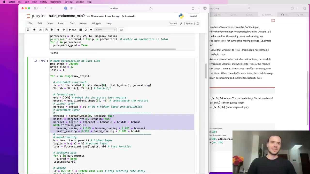
Nobody wants a second stage, so the paper also proposes estimating the statistics on the side during training (56:03). bnmean_running starts at zeros and bnstd_running at ones, matching what Kaiming-scaled pre-activations look like at the start (57:04). Each step nudges them, 0.999 old plus 0.001 new, inside torch.no_grad() because these are not trained by gradient descent (58:07). After training the running values closely match the calibrated ones, and the validation loss is basically identical (1:00:13).
1:00:46 – 1:04:58 Epsilon, the useless bias, and a recap
Two details. The paper’s ε, by default 1e-5, sits under the square root so a batch with zero variance can’t cause division by zero (1:00:46). And the bias b1 in the linear layer is now dead weight (1:01:17): whatever constant it adds, the mean subtraction removes, so its gradient is zero. Drop it and let BatchNorm’s own bias do the job (1:01:48). Keeping it does no harm, just wastes parameters.
The recap (1:02:52) separates two kinds of state. The gain and bias are parameters trained with backprop. The running mean and standard deviation are buffers, updated by the moving average and used at inference.
1:04:58 – 1:14:18 BatchNorm in the wild: ResNet and PyTorch’s layers
A look at PyTorch’s ResNet code shows the same pattern at scale (1:04:58). The bottleneck block stacks convolution, batch norm, ReLU, repeated, plus residual connections still to be covered. Karpathy explains a convolution as wx + b applied to overlapping patches of an image (1:06:00), and points out that the convolutions use bias=False for exactly the reason just discussed (1:07:34).
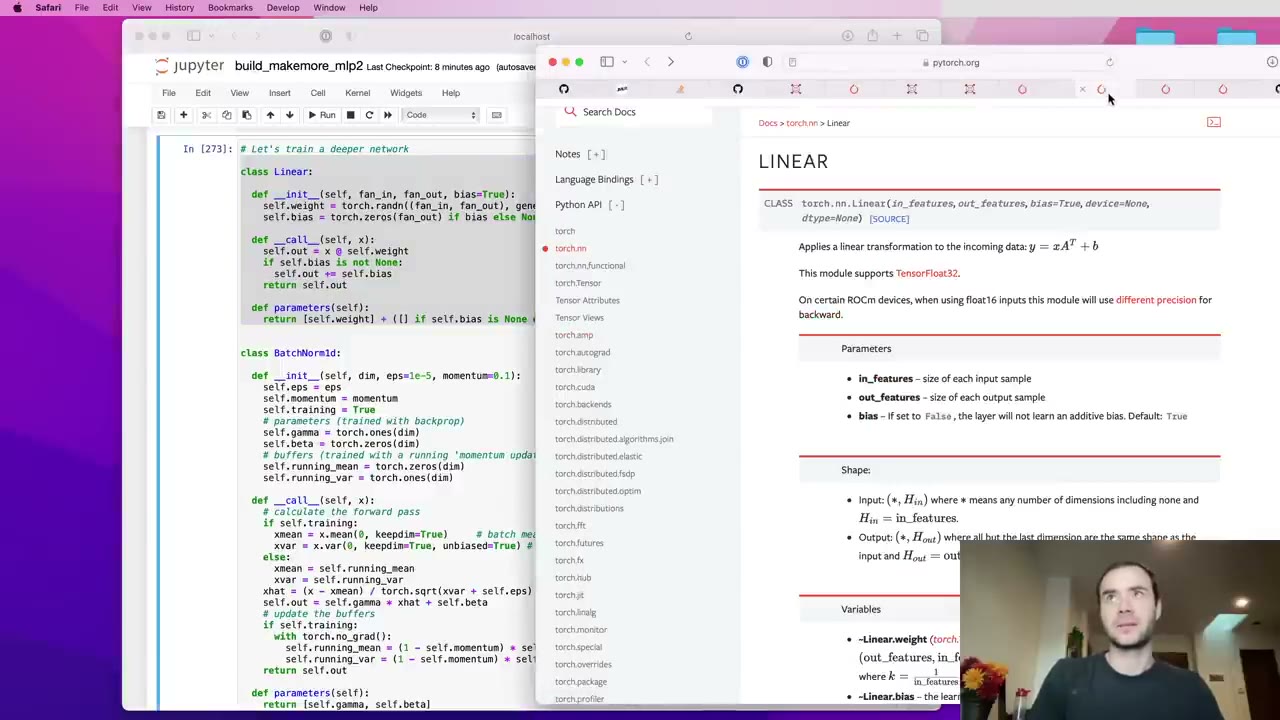
He then reads two documentation pages. nn.Linear takes fan-in, fan-out and a bias flag (1:09:06), and by default draws weights uniformly with scale 1/√fan_in, the same idea with a gain of 1 (1:10:09). nn.BatchNorm1d takes the number of features, eps and momentum (1:11:10). PyTorch’s default momentum of 0.1 is fine for large batches, but with batches of 32 the batch statistics bounce around, and the running estimate may thrash instead of settling, which is why the lecture used 0.001 (1:12:14). affine controls the learned gain and bias, track_running_stats lets you skip the moving average if you plan to calibrate afterwards (1:13:16).
1:14:18 – 1:18:30 The first wrap-up
Karpathy summarizes the argument so far (1:14:18): fix overconfident outputs to avoid the hockey stick, keep activations roughly Gaussian throughout, scale weights to get there, and use a normalization layer once the network is too deep to scale by hand. Then a personal warning: he has been burned by BatchNorm bugs many times himself (1:16:57), and recommends avoiding BatchNorm where possible in favor of layer or group normalization (1:17:29). The lecture appears to end, pointing ahead to RNNs as very deep networks once unrolled (1:18:00).
1:18:30 – 1:26:49 PyTorch-ifying the code into modules
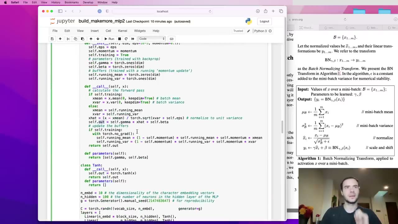
Then Karpathy admits the ending was premature and starts a bonus section (1:18:30). The code is restructured into classes that mirror torch.nn. Linear holds a weight initialized with 1/√fan_in and an optional zero bias (1:19:31). BatchNorm1d takes dim, eps and momentum (1:20:32) and has a training flag (1:21:35), because in training it uses batch statistics and updates its buffers, while in eval it uses the frozen running values. This version follows the paper and tracks variance rather than standard deviation (1:23:07). Each module also stores its output in .out, a non-PyTorch addition purely for plotting (1:23:38). Tanh has no parameters.
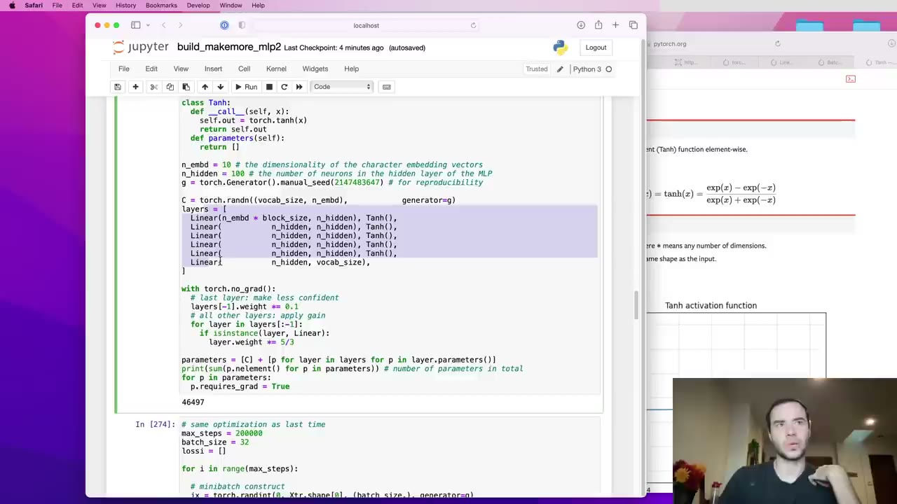
With layers as objects, a six-layer MLP is just a list: linear, tanh, linear, tanh, and so on (1:25:13), about 46,000 parameters. The training loop calls retain_grad() on every layer’s output so the gradients of these intermediate tensors can be inspected after backward() (1:26:18).
Our note: Karpathy’s x.var(0, keepdim=True) uses PyTorch’s default unbiased estimate (dividing by n − 1; the first version on screen spells out unbiased=True), while PyTorch’s own nn.BatchNorm1d normalizes with the biased one. The difference is small at batch size 32, and Lecture 5 returns to it.
1:26:49 – 1:36:15 Histograms across six layers, and the linear sandwich
The first diagnostic plots the distribution of each tanh layer’s output after one step, with mean, standard deviation and the percentage of values beyond 0.97 (1:26:49). With a gain of 5/3 the first layer is about 20% saturated, and deeper layers settle around a standard deviation of 0.65 and about 5% saturation (1:27:50).
Turning the gain knob shows why it matters:
| Gain on linear layers | What happens (tanh network) |
|---|---|
| 1 | Activations shrink layer by layer toward zero (1:28:53) |
| 5/3 | Stable spread, about 5% saturation |
| 3 | Far too saturated (1:29:58) |
Karpathy says plainly that he doesn’t know where 5/3 came from (1:30:30); it just works empirically. The same plot for gradients should show every layer with roughly the same spread (1:31:01). Too small a gain, such as 0.5, or too large, such as 3, and the gradient histograms drift apart from layer to layer.
He then deletes every tanh (1:32:04). With a gain of 5/3 the activations spread out layer by layer while the gradients shrink going down; the correct gain for pure linear layers is 1 (1:33:39). Before normalization layers, Adam and residual connections, training deep nets meant precisely orchestrating all of this (1:34:09). Why keep tanh at all, then? A stack of linear layers collapses to a single linear function in the forward pass (1:34:40), although its training dynamics differ (1:35:13). The nonlinearity is what lets the network approximate arbitrary functions.
1:36:15 – 1:46:07 Weight gradients and the update-to-data ratio
The third plot covers the parameters themselves (1:36:15), restricted to 2-D weight matrices. For each it prints the gradient’s mean and standard deviation and the grad-to-data ratio, the scale of the gradient relative to the weights (1:37:48). Most are around 1e-3, but the last layer’s gradients are about ten times larger than the rest (1:38:51), so plain SGD would train it about ten times faster at the start. After 1,000 steps it partly evens out.
Karpathy prefers a more direct measure (1:39:55): the update-to-data ratio, the standard deviation of lr * grad divided by that of the weights, logged as log10 at every step. Plotted over time against a guide line at −3 (1:41:58), it says how much each step changes each tensor. The last layer starts as an outlier only because it was shrunk by 0.1 to calm the softmax (1:42:30).
The plot doubles as a learning-rate check. At lr = 0.001 every update is about 10,000 times smaller than the weights, a sign of training far too slowly (1:43:32). The current setting sits near −2.5, slightly high but fine (1:44:02). Forget the √fan_in scaling and every plot goes wrong at once: saturated activations, messy gradients, and update ratios around −1 to −1.5 (1:45:05).
1:46:07 – 1:51:23 BatchNorm in the deep network
All this tuning feels like “balancing of a pencil on your finger” (1:46:07), so BatchNorm goes in after each linear layer and before the tanh (1:46:37). Placing it after the nonlinearity gives similar results, and one after the last linear layer is fine too, in which case the softmax is calmed by shrinking that layer’s gamma instead of its weights (1:47:10).
The activations are now healthy by construction: about 0.65 standard deviation and 2% saturation in every layer (1:47:42). Set the gain to 0.2 and the activations don’t change at all, but the update ratios do, because the scale of the incoming activations interacts with BatchNorm’s backward pass (1:48:44). Drop the √fan_in scaling entirely and the forward and backward plots still look good, but updates fall well below −3 (1:49:47), so the learning rate needs about a tenfold increase, to 1.0 (1:50:18). The weight scale no longer matters much; the learning rate still does.
1:51:23 – end Three goals, and what’s left unsolved
Karpathy lists what the lecture set out to do (1:51:23): introduce batch normalization, PyTorch-ify the code so that prefixing the classes with nn. would run against real PyTorch (1:51:54), and teach the diagnostic plots, viewed over time rather than as single snapshots (1:52:55).
What it didn’t do (1:53:27): beat the previous loss. He tried a BatchNorm network off camera and got about the same result, because the model is no longer limited by optimization but by its three-character context (1:53:58), which calls for RNNs and transformers. He also didn’t fully explain why, say, changing the gain changes the right learning rate. That needs a close look at every layer’s backward pass (1:54:29), and initialization and update rules remain open research problems (1:55:00).
Our note: the backward pass of every layer here, BatchNorm included, is exactly what Lecture 5 works through by hand.
Code you’ll write
Sanity checks for initialization. Compute the loss a clueless model should get, then look at how many tanh units are stuck in the tails (18:36).
# expected loss at init: uniform over 27 characters
-torch.tensor(1/27.0).log()   # tensor(3.2958)

# distribution of hidden activations, and where they saturate
plt.hist(h.view(-1).tolist(), 50);
plt.figure(figsize=(20, 10))
plt.imshow(h.abs() > 0.99, cmap='gray', interpolation='nearest')
The fixed initialization. Zero output bias, small output weights, and Kaiming scaling for the tanh layer, with fan-in 30 (39:29).
n_embd = 10     # dimensionality of each character embedding
n_hidden = 200  # neurons in the hidden layer

g = torch.Generator().manual_seed(2147483647)
C  = torch.randn((vocab_size, n_embd),            generator=g)
W1 = torch.randn((n_embd * block_size, n_hidden), generator=g) * (5/3)/((n_embd * block_size)**0.5)
b1 = torch.randn(n_hidden,                        generator=g) * 0.01
W2 = torch.randn((n_hidden, vocab_size),          generator=g) * 0.01
b2 = torch.randn(vocab_size,                      generator=g) * 0
BatchNorm inline, with running statistics. Standardize the pre-activations over the batch, apply the learned gain and bias, and update the running estimates outside autograd (57:04). b1 is gone, since BatchNorm would cancel it.
bngain = torch.ones((1, n_hidden))
bnbias = torch.zeros((1, n_hidden))
bnmean_running = torch.zeros((1, n_hidden))
bnstd_running = torch.ones((1, n_hidden))

# inside the training loop
hpreact = embcat @ W1  # no bias: BatchNorm subtracts it anyway
bnmeani = hpreact.mean(0, keepdim=True)
bnstdi = hpreact.std(0, keepdim=True)
hpreact = bngain * (hpreact - bnmeani) / bnstdi + bnbias
with torch.no_grad():
  bnmean_running = 0.999 * bnmean_running + 0.001 * bnmeani
  bnstd_running = 0.999 * bnstd_running + 0.001 * bnstdi
A BatchNorm1d module. The forward pass of the PyTorch-style class; __init__ sets gamma to ones, beta to zeros, and the running mean and variance to zeros and ones (1:20:32).
def __call__(self, x):
  if self.training:
    xmean = x.mean(0, keepdim=True)  # batch mean
    xvar = x.var(0, keepdim=True)    # batch variance
  else:
    xmean = self.running_mean
    xvar = self.running_var
  xhat = (x - xmean) / torch.sqrt(xvar + self.eps)  # normalize to unit variance
  self.out = self.gamma * xhat + self.beta
  if self.training:
    with torch.no_grad():
      self.running_mean = (1 - self.momentum) * self.running_mean + self.momentum * xmean
      self.running_var = (1 - self.momentum) * self.running_var + self.momentum * xvar
  return self.out
A six-layer tanh MLP with a gain. Stack modules in a list, calm the output layer, and boost every hidden linear layer by 5/3 (1:25:13). The BatchNorm version adds BatchNorm1d(n_hidden) after each Linear, passes bias=False, and shrinks layers[-1].gamma instead.
n_hidden = 100  # the deep network uses 100 hidden units
layers = [
  Linear(n_embd * block_size, n_hidden), Tanh(),
  Linear(           n_hidden, n_hidden), Tanh(),
  Linear(           n_hidden, n_hidden), Tanh(),
  Linear(           n_hidden, n_hidden), Tanh(),
  Linear(           n_hidden, n_hidden), Tanh(),
  Linear(           n_hidden, vocab_size),
]
with torch.no_grad():
  layers[-1].weight *= 0.1  # last layer: make less confident
  for layer in layers[:-1]:
    if isinstance(layer, Linear):
      layer.weight *= 5/3
parameters = [C] + [p for layer in layers for p in layer.parameters()]
Tracking the update-to-data ratio. Log, at every step, how big each update is relative to the tensor it changes, then plot it for the weight matrices against the −3 guide line (1:40:26).
# in the training loop, after the update
with torch.no_grad():
  ud.append([((lr*p.grad).std() / p.data.std()).log10().item() for p in parameters])

# after training
plt.figure(figsize=(20, 4))
for i, p in enumerate(parameters):
  if p.ndim == 2:
    plt.plot([ud[j][i] for j in range(len(ud))])
plt.plot([0, len(ud)], [-3, -3], 'k')  # ratios should be ~1e-3
The complete notebook for this lecture, including the histogram cells and sampling code, is makemore_part3_bn.ipynb in the MIT-licensed nn-zero-to-hero repo. The standalone makemore repo has the full character-level model in script form.
Skip list
- 0:02 – 4:10 Walkthrough of the cleaned-up Lecture 3 code. Skip if you just watched Lecture 3; the only new piece is
@torch.no_grad(). - 1:04:58 – 1:09:06 Tour of PyTorch’s ResNet code. Useful context, but the only point for this lecture is
bias=Falsebefore batch norm. - 1:14:18 – 1:18:30 The first summary, which repeats the lecture so far before the bonus section begins.
- 1:53:27 – end Closing reflections on what wasn’t covered.
Glossary
- Logits — the raw scores the last layer outputs, before softmax turns them into probabilities.
- Hockey-stick loss — a loss curve with a steep drop in the first steps, a sign the model started out overconfident and spent early training just shrinking its outputs.
- Saturation — a squashing unit such as tanh operating in its flat tails, where its local gradient is close to zero.
- Dead neuron — a unit that is saturated, or for ReLU switched off, for every input, so it never receives gradient and never learns.
- Fan-in — the number of inputs feeding each unit of a layer; Kaiming scaling divides by its square root.
- Gain — a factor on top of 1/√fan_in that compensates for how much a nonlinearity squashes its input: 1 for linear, √2 for ReLU, 5/3 for tanh.
- Kaiming (He) initialization — drawing weights with standard deviation gain / √fan_in so activations keep roughly unit variance through depth.
- Batch normalization — a layer that standardizes each unit’s pre-activation over the batch, then rescales and shifts it with a learned gain (gamma) and bias (beta).
- Buffers — a layer’s state that is not trained by gradient descent, such as BatchNorm’s running mean and variance.
- Momentum (BatchNorm) — the weight given to the newest batch when updating the running statistics; high values suit large batches, low values small ones.
- Epsilon (BatchNorm) — a small constant added to the variance to avoid division by zero.
- Train / eval mode — the switch that tells layers like BatchNorm whether to use batch statistics and update buffers, or use the frozen running values.
- Grad-to-data ratio — the scale of a parameter’s gradient compared with the scale of the parameter itself.
- Update-to-data ratio — the scale of the actual step (learning rate times gradient) compared with the parameter; around 1e-3 per step is Karpathy’s rule of thumb.
FAQ
Why is the first loss 27 in makemore Part 3, and what should it be?
With 27 possible next characters and no knowledge yet, the network should spread its probability evenly, which gives a loss of -log(1/27), about 3.29. The starting MLP instead produces large, random logits, so it is confidently wrong on most examples. Karpathy fixes it by setting the output bias to zero and scaling the output weights down by 0.01, which removes the hockey-stick shape from the loss curve and improves the final validation loss.
Where does the 5/3 gain for tanh come from?
Karpathy says in the lecture that he does not know where PyTorch's 5/3 comes from. He shows empirically that it works: in a stack of linear and tanh layers it keeps activations from shrinking or saturating, with about 5% of tanh units in the tails. Our note: 5/3 is the value PyTorch's torch.nn.init.calculate_gain returns for tanh, and it multiplies the 1/sqrt(fan_in) scale used in Kaiming initialization.
Why do you remove the bias from a layer that feeds into BatchNorm?
BatchNorm subtracts each neuron's batch mean, so any constant bias added just before it is subtracted straight back out. The bias then gets zero gradient and never learns. BatchNorm has its own learnable bias (beta), so the earlier one is simply wasted parameters. That is why the ResNet code Karpathy shows passes bias=False to the convolutions that precede batch norm.
How does BatchNorm work at test time when there is only one example?
During training BatchNorm normalizes with the current batch's mean and standard deviation, which a single example can't provide. The fix is to use fixed statistics at inference. You can measure them over the whole training set after training, or, as PyTorch does, keep an exponential running average during training and switch to it in eval mode. Karpathy shows the two give nearly identical numbers.
What update-to-data ratio should a healthy network have?
Karpathy's rough rule of thumb is that each step's update should be about one thousandth of the size of the weights it changes, around -3 on a log10 plot. Much lower suggests the learning rate is too small and training is slow; much higher suggests updates are too large. He tracks the ratio for every weight matrix over the first steps of training rather than at a single moment.
Studying another course? Paste its YouTube or Bilibili link on the home page to request a handout — or make your own with the desktop app (coming soon).