Karpathy's Zero to Hero, Lecture 5: Becoming a Backprop Ninja — notes, code and timestamps
 0:41
 1:12
 2:33
 3:56
 4:14
 4:30
 5:34
 6:00
 6:23
 6:33
 7:42
 8:01
 9:25
 10:19
 10:39
 11:42
 13:15
 14:30
 16:45
 18:52
 19:45
 22:01
 22:46
 23:15
 25:14
 26:26
 28:16
 29:47
 32:30
 34:51
 37:30
 39:35
 40:40
 41:40
 41:57
 43:45
 48:29
 53:20
 54:11
 55:55
 58:42
 59:57
 1:02:27
 1:03:24
 1:04:16
 1:05:31
 1:06:52
 1:07:13
 1:08:28
 1:10:23
 1:13:45
 1:16:30
 1:18:22
 1:19:04
 1:21:22
 1:22:12
 1:26:23
 1:27:51
 1:28:37
 1:30:11
 1:32:25
 1:33:04
 1:35:19
 1:37:28
 1:38:25
 1:40:59
 1:42:55
 1:45:39
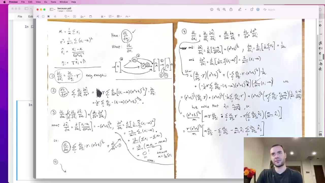 1:47:20
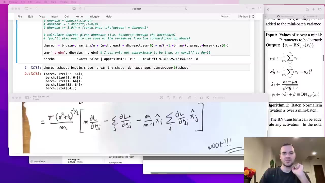 1:48:37
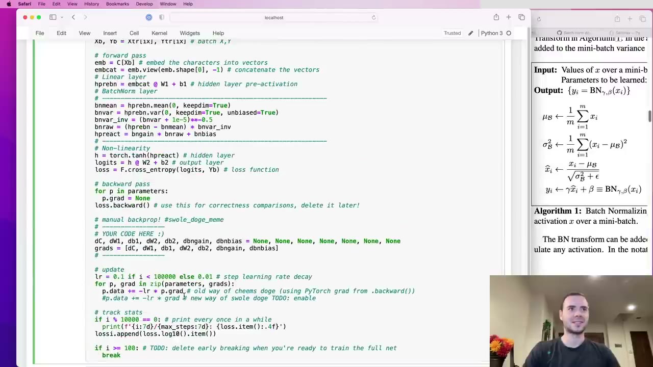 1:50:53
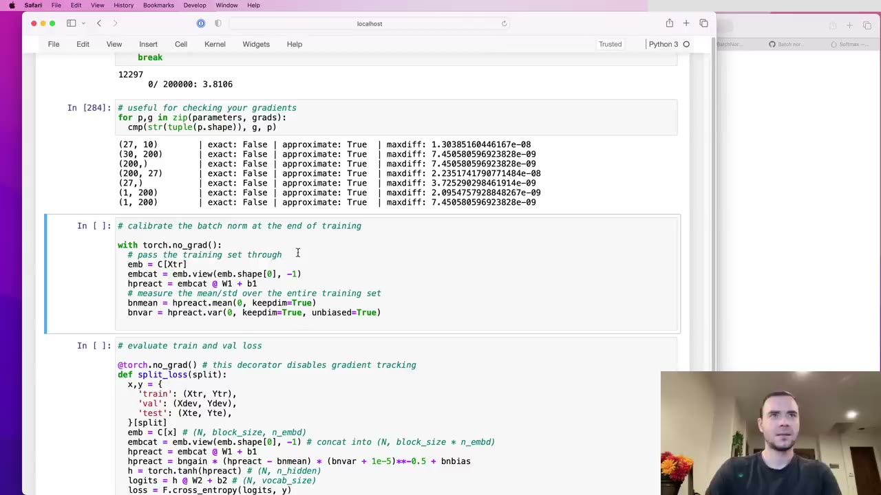 1:51:43
 1:52:14
 1:53:42
 1:53:48
 1:54:26
Watch the video (115 min)
Watch the original video on YouTube
Lecture 5 of Andrej Karpathy’s Neural Networks: Zero to Hero is the one where nothing new gets built. The model is the same character-level MLP with a BatchNorm layer from Lecture 4. What changes is that loss.backward() is deleted. In its place, Karpathy derives and writes every gradient himself, tensor by tensor, from the loss all the way back to the embedding table, and checks each one against PyTorch. It is the tensor-level sequel to micrograd: the same chain rule, but with broadcasting, sums and matrix multiplies in the way. The lecture is organised as four exercises: backpropagate through a deliberately long, chunked forward pass; replace the cross-entropy chain with one derived formula; do the same for BatchNorm; then train the network with only your own gradients. Next comes Lecture 6, where the architecture finally starts to grow. For the whole course, see the series index.
Key takeaways
- Backprop is a leaky abstraction (1:05). Autograd computes gradients for you, but saturated activations, dead neurons and subtle bugs only make sense if you know what it is computing.
- A gradient always has the shape of the thing it belongs to (12:55). Checking shapes first catches most mistakes before any calculus.
- Sums and broadcasts are each other’s backward pass (1:09:32). A sum along a dimension in the forward pass becomes a broadcast along it in the backward pass, and a broadcast (a reused value) becomes a sum.
- When a tensor feeds two branches, its gradients add (27:25). Several intermediates get their first gradient early and the rest later, so the second contribution uses
+=. - You don’t need to memorize matrix-multiply gradients (49:41). Write out a 2×2 case once, then let the shapes tell you where the transpose goes.
- The cross-entropy gradient is softmax minus one-hot (1:30:34). It pulls the wrong characters down and the right one up, with forces that balance exactly.
- BatchNorm’s backward pass collapses to one line (1:48:38), but deriving it on paper means tracking which quantities are vectors and which are single numbers.
- Manual gradients train the same network (1:53:20). With
loss.backward()gone, the loss and samples come out much as before.
Chapter notes
0:02 – 3:40 Why backprop is a leaky abstraction
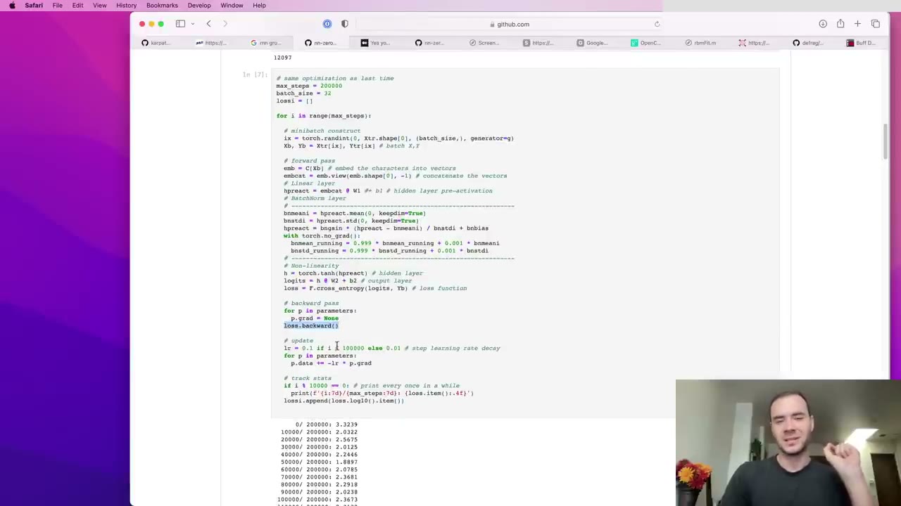
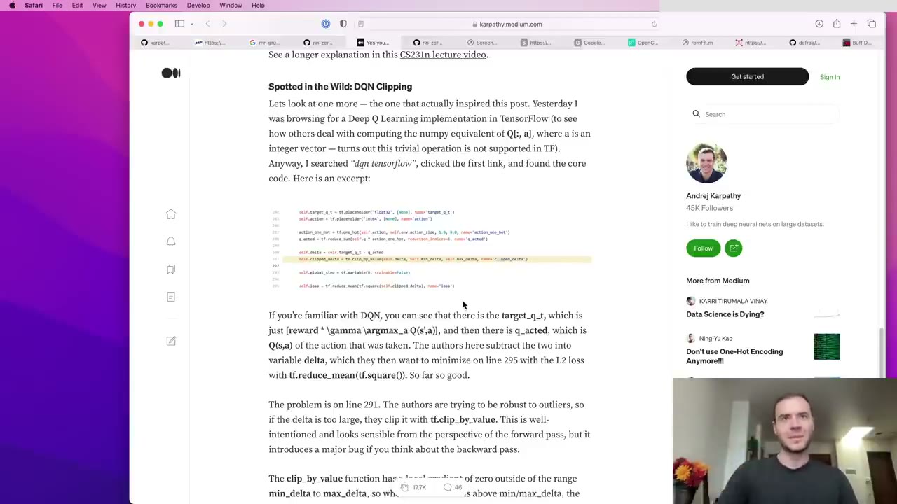
Karpathy opens by admitting that everyone wants to get on to recurrent networks, and that he is holding the class back for one more lecture. The line he objects to is loss.backward(). Leaning on autograd is fine for daily work, but he argues it hides things that bite: flat tails of squashing functions that kill gradients, dead neurons, exploding or vanishing gradients in recurrent networks (1:36). His real-world example is a snippet that clips the loss at a maximum value when the author meant to clip gradients (2:07). Clipping a loss sets an outlier’s gradient to zero, so those examples are silently ignored.
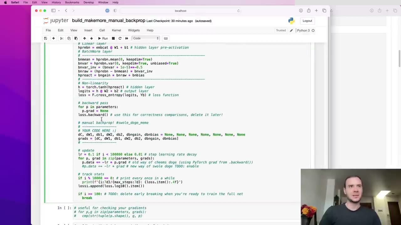
loss.backward() highlighted. This is the one line the lecture sets out to replace.
clip_by_value zeroes the gradient for outliers instead of capping it.micrograd already covered the chain rule, but on single numbers. This lecture moves the same reasoning up to tensors, which is where real code lives.
Our note: the blog post he mentions is his 2016 essay “Yes you should understand backprop”.
3:40 – 7:15 When everyone wrote the backward pass by hand
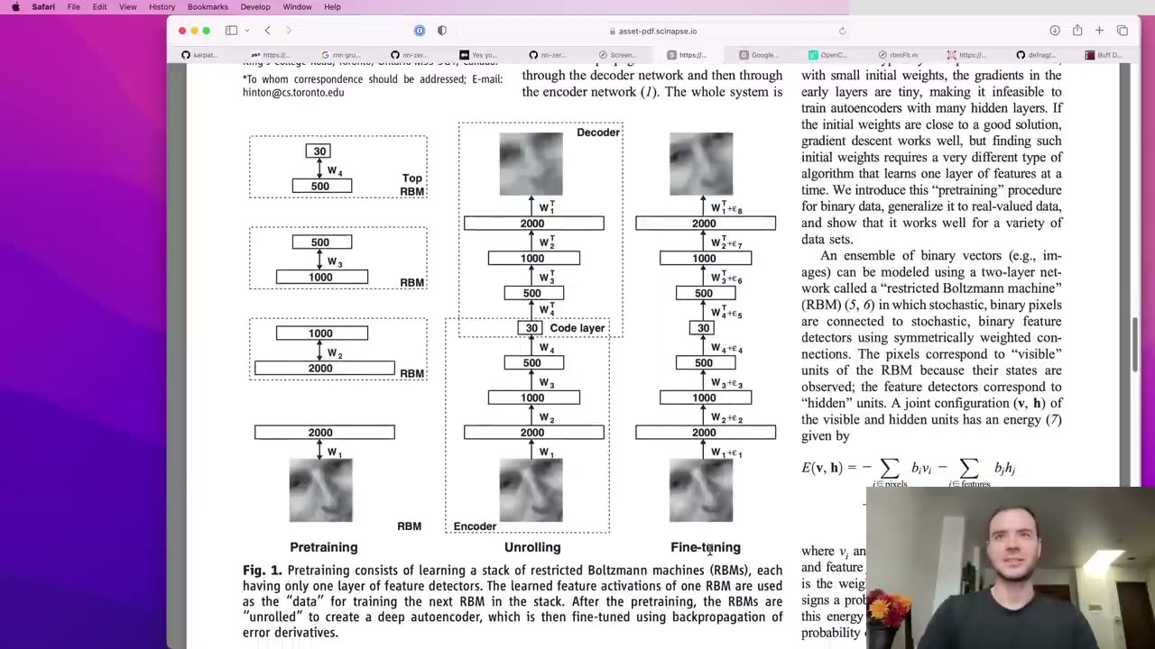
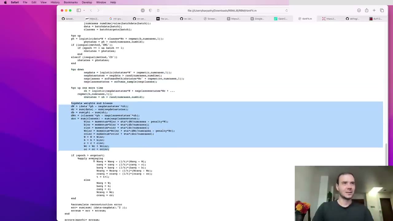
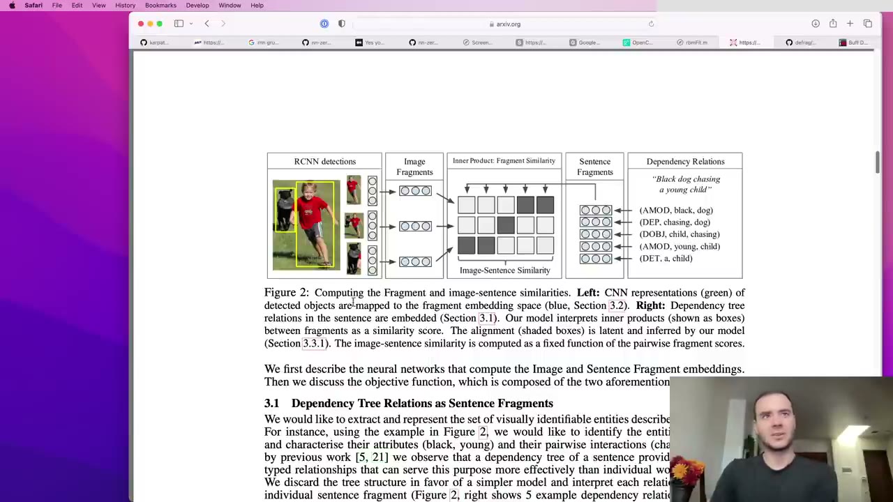
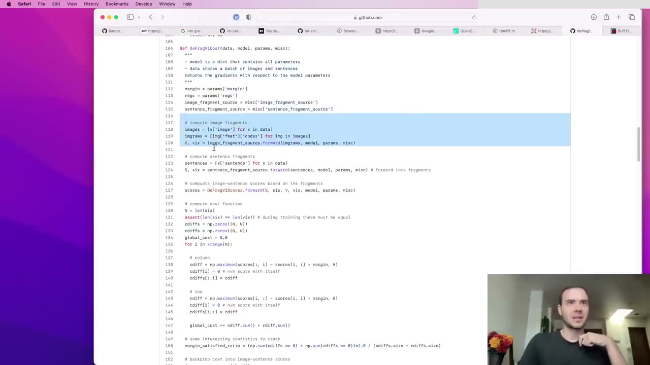
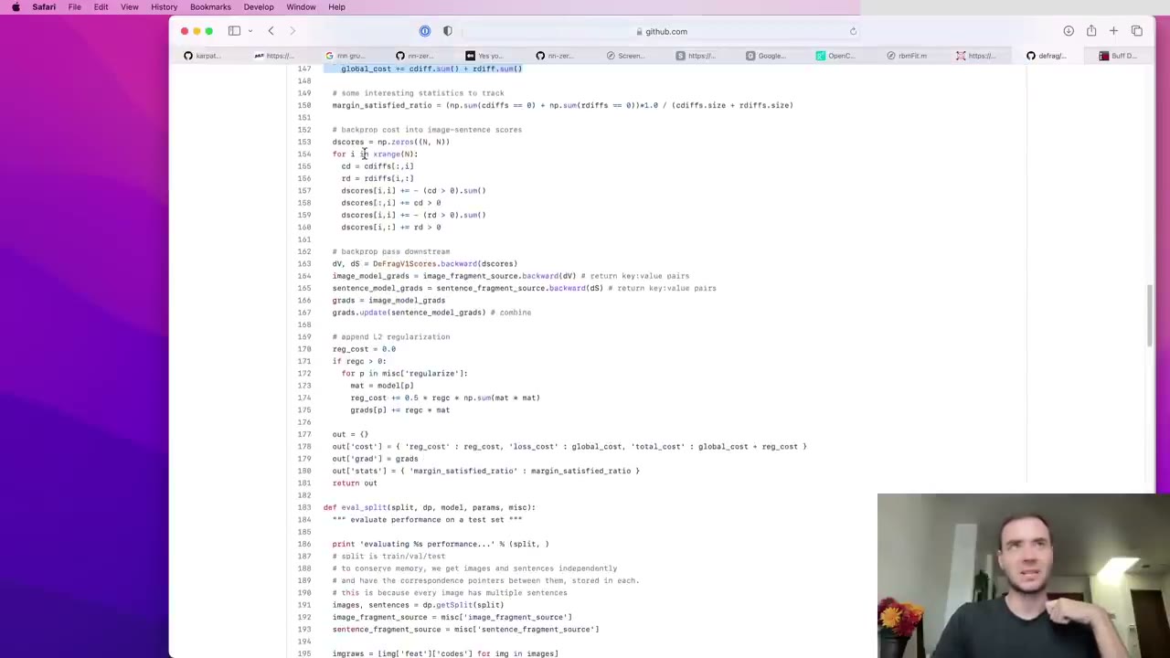
A short history detour. About a decade before this video, writing your own backward pass was standard practice. He shows Hinton and Salakhutdinov’s 2006 Science paper on restricted Boltzmann machines, his own Matlab code from around 2010 for training them (4:41), where gradients are estimated and applied inline, and the NumPy code behind his 2014 fragment-embeddings paper, which aligned image regions with pieces of sentences in a CLIP-like way (5:41). There the cost function and its backward pass sat side by side, and a numerical gradient checker confirmed them. His view: people understood their networks more intuitively when they had to do this.
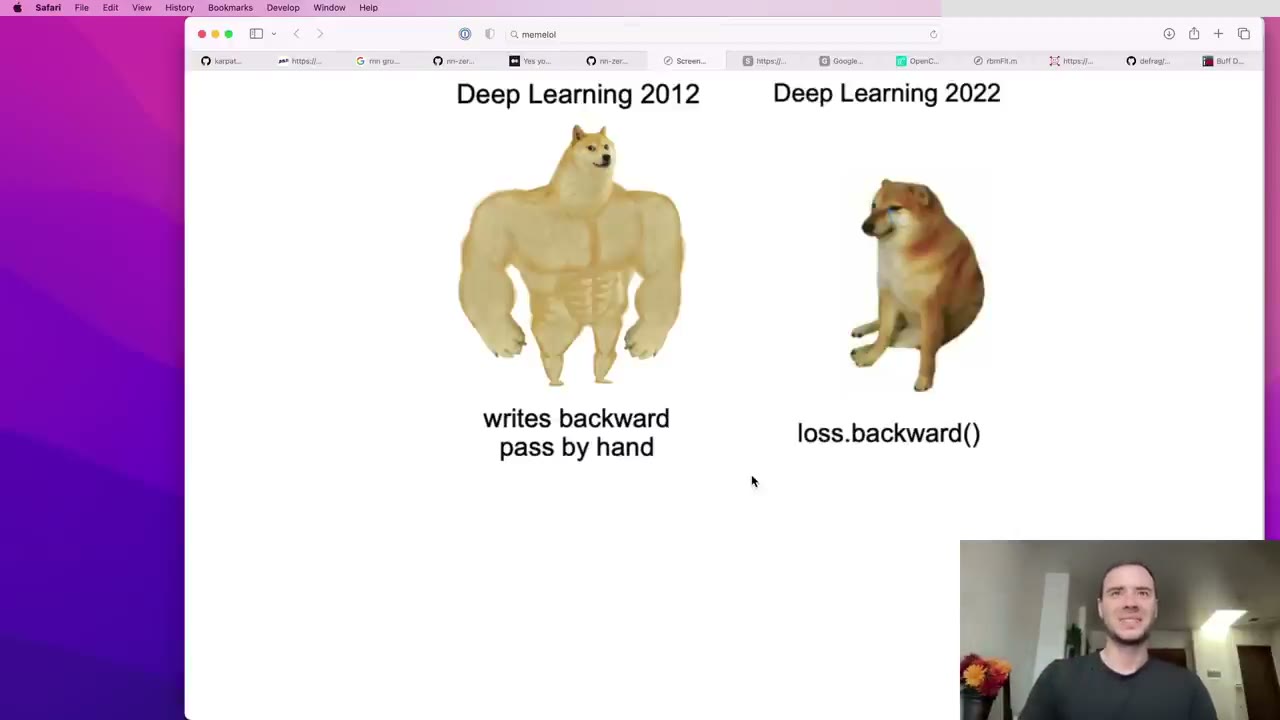
loss.backward().
7:15 – 12:23 The starter notebook and the four exercises
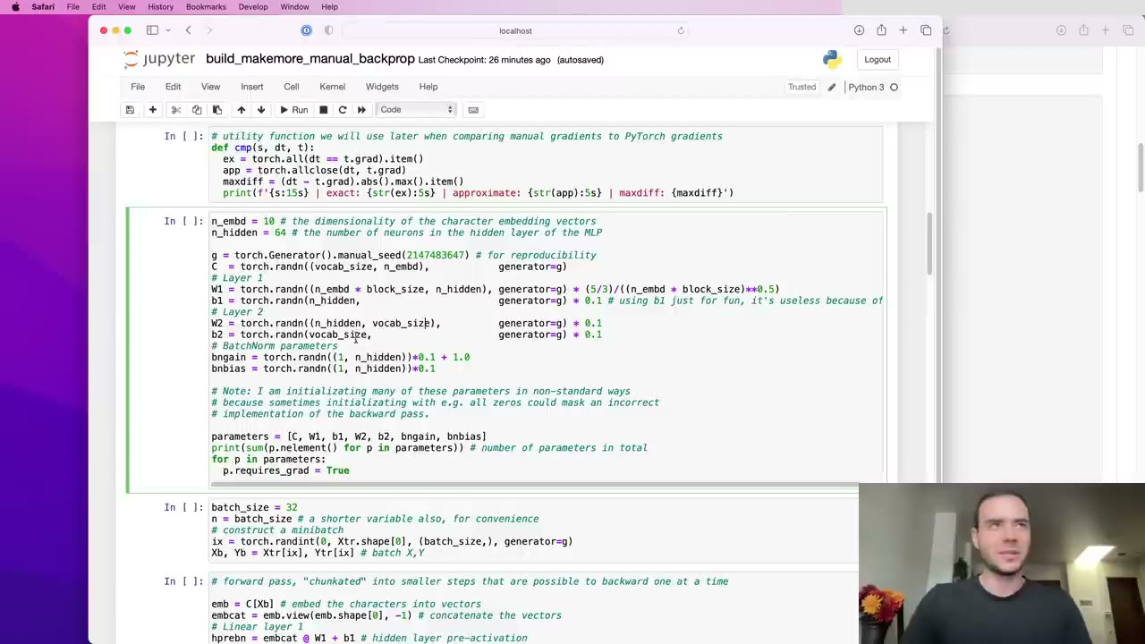
The setup is unchanged: same data, same two-layer MLP with BatchNorm in between. Three things are new (7:46):
- A
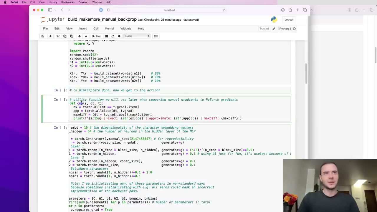
cmphelper that compares a hand-computed gradient with PyTorch’s.grad, reporting exact equality, approximate equality (torch.allclose) and the largest absolute difference. - Small random biases instead of zeros (8:18). Zero values can make a wrong gradient formula look right, because many terms vanish. He also keeps a bias
b1before BatchNorm, which is pointless for the model but gives one more gradient to check. - A long forward pass (9:19).
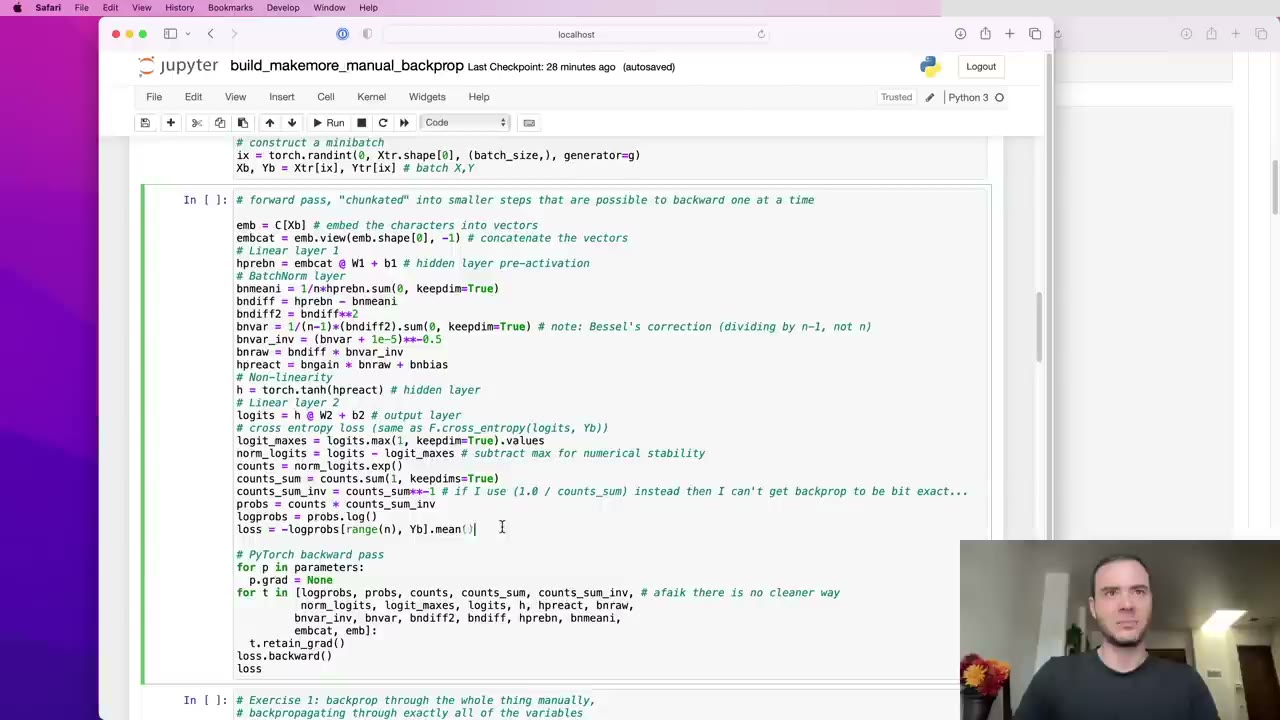
F.cross_entropyis replaced by an explicit softmax and negative log likelihood, and BatchNorm is split into one operation per line, so every intermediate tensor can be backpropagated through on its own. Each will get a matchingd-prefixed gradient:logprobsgetsdlogprobs, and so on.
cmp helper: exact match, torch.allclose, and the largest absolute difference against PyTorch's .grad.
retain_grad() on every intermediate so PyTorch's gradients are available for checking.He previews the plan (10:20) and recommends opening the notebook or its Colab copy and trying each gradient yourself before watching him do it (12:23).
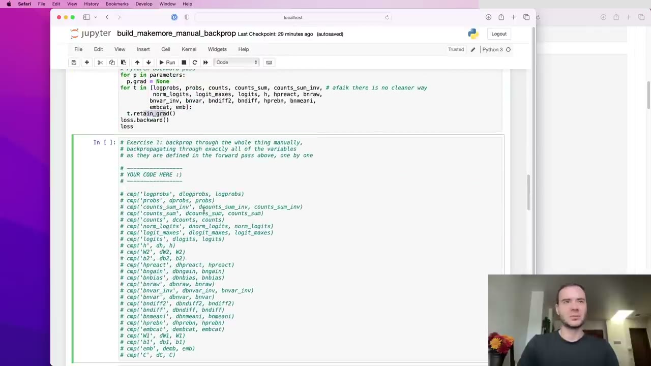
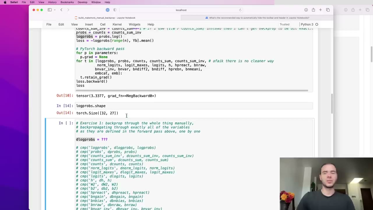
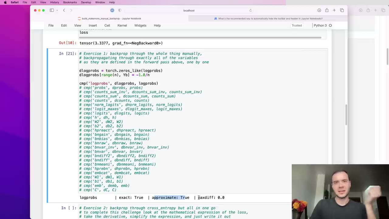
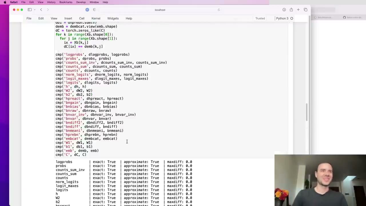
cmp call per intermediate, from logprobs down to the embedding table C.
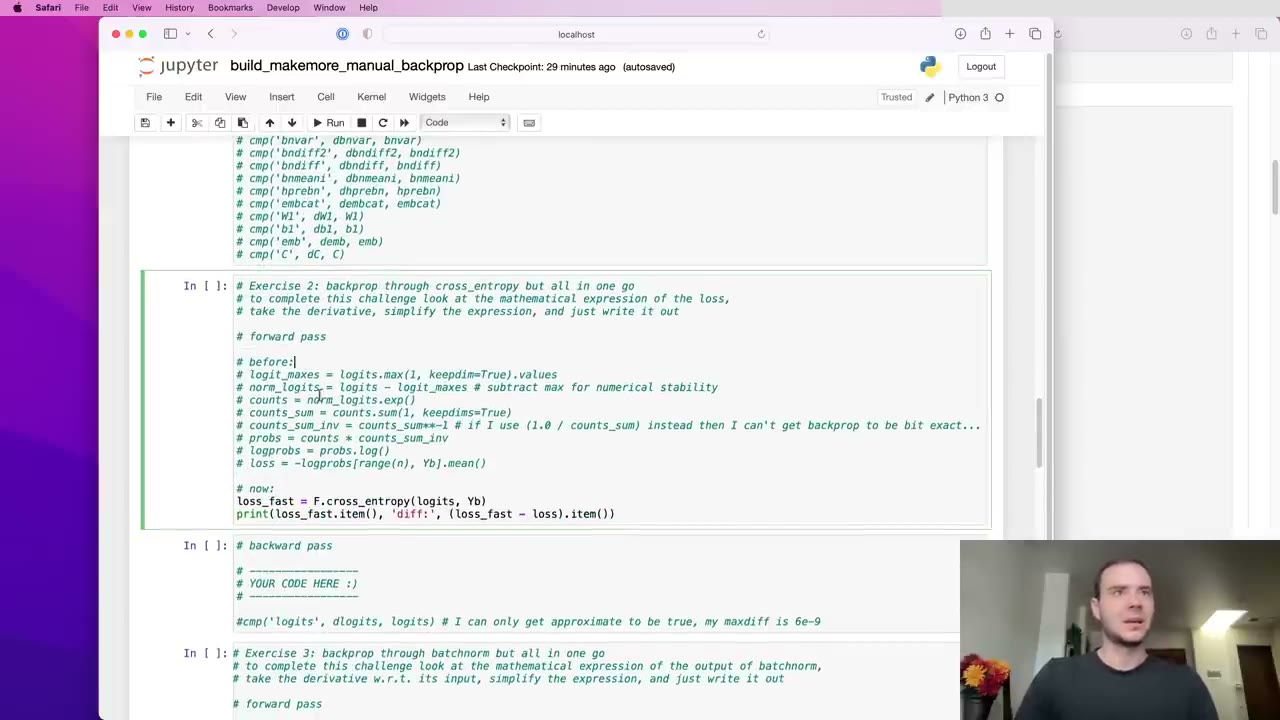
F.cross_entropy, and the backward pass is left for you to derive.
p.grad.12:23 – 20:41 First gradients: dlogprobs and dprobs
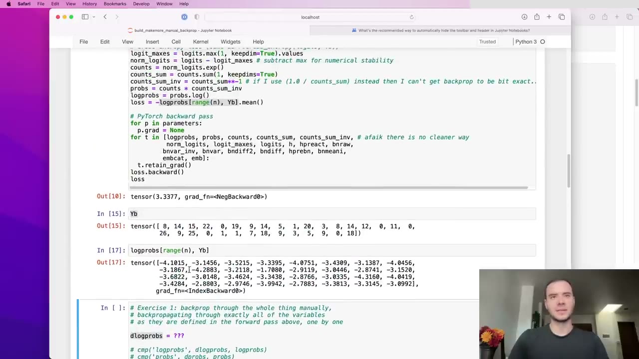
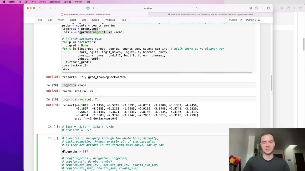
The loss is the negative mean of 32 entries plucked out of the 32×27 logprobs tensor, one per row at the correct next character. A three-number toy version makes the derivative obvious (14:58): each plucked entry gets −1/n, and the other 832 entries get exactly zero because they never touch the loss. The code is a tensor of zeros with −1/n written into those positions, and cmp reports an exact match (18:35).
logprobs is 32×27, so dlogprobs must be too.
range(n) and Yb pulls out one log probability per row, the ones the loss actually uses.
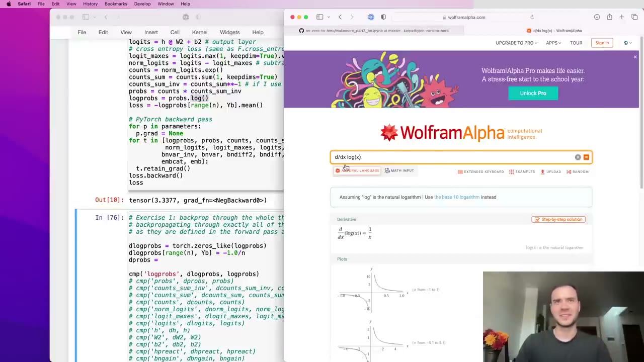
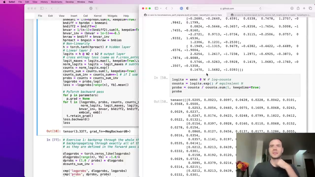
The next step goes through an element-wise log (19:06). The local derivative is 1/x, so dprobs is dlogprobs / probs. He points out what that means: where the network already gives the right character a probability near 1, the gradient passes through almost unchanged; where it gives it a low probability, the gradient is boosted (20:08).
dprobs = (1.0 / probs) * dlogprobs.20:41 – 32:36 Through the softmax: broadcasting and its backward sum
A quick recap of how the forward pass builds probabilities: subtract each row’s maximum for stability, exponentiate into counts, sum each row, invert, multiply. He uses counts_sum**-1 instead of a division because, he says, PyTorch’s division backward didn’t give him a bit-exact match (21:43).
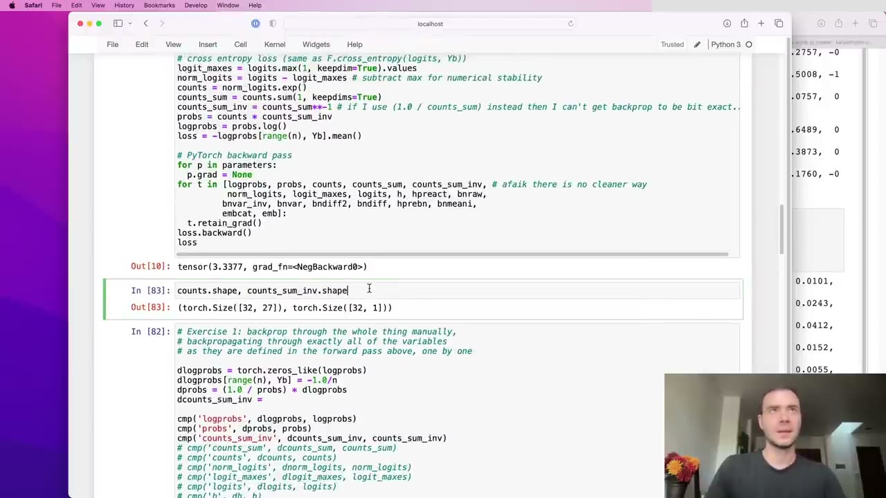
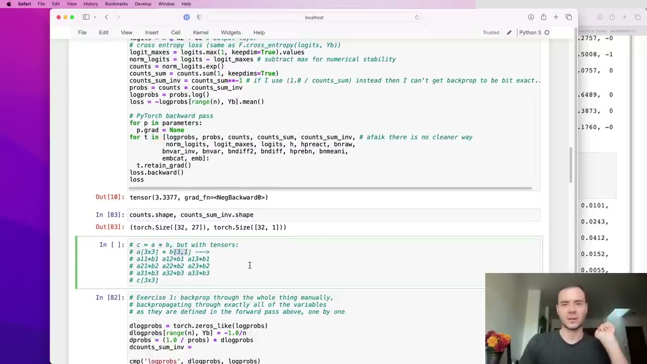
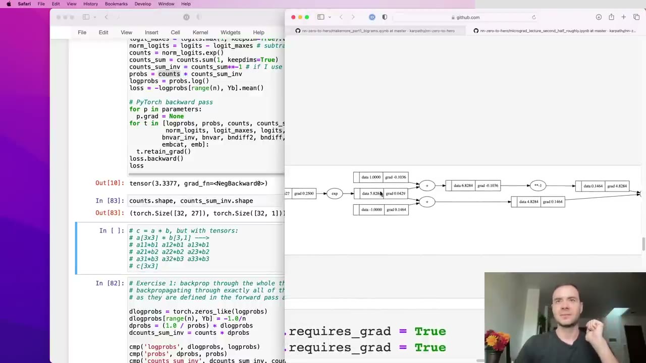
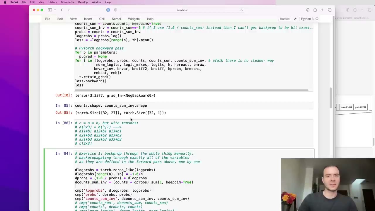
The line probs = counts * counts_sum_inv is the first real trap. counts is 32×27 but counts_sum_inv is 32×1, so PyTorch silently copies the column 27 times before multiplying. Karpathy treats that as two operations (23:17): a replication, then an element-wise multiply. The multiply’s gradient is the other factor times dprobs. The replication means one value was reused 27 times, and as in micrograd, gradients from every use add up (25:22). So the result is summed across each row, with keepdim=True to keep the 32×1 shape.
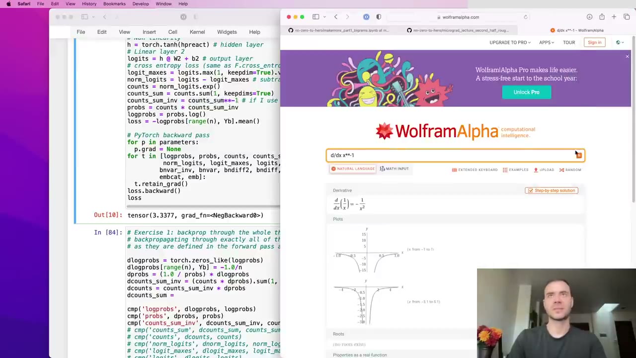
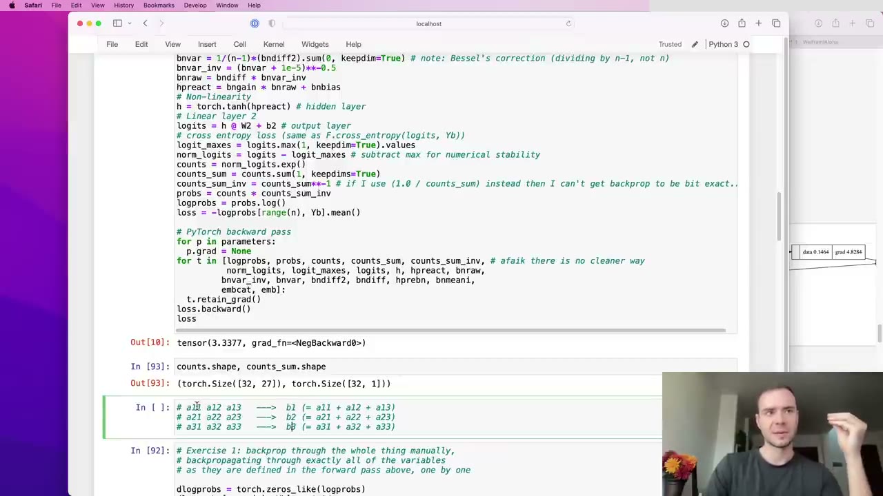
counts has the same problem from the other side: it feeds probs directly and also feeds counts_sum. Its first gradient can’t be checked yet (27:25). The power rule handles counts_sum (27:55), and the row sum is undone by spreading each row’s gradient back across all 27 columns (30:32). His phrase for this: addition is a router of gradient. Adding this second contribution with += makes dcounts match (32:05).
counts_sum**-1.
counts, added with +=.32:36 – 41:51 Exponentials, the stability branch and F.one_hot
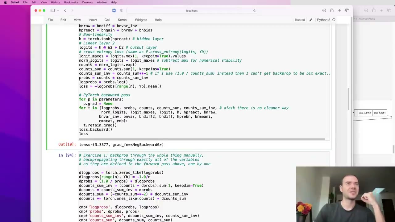
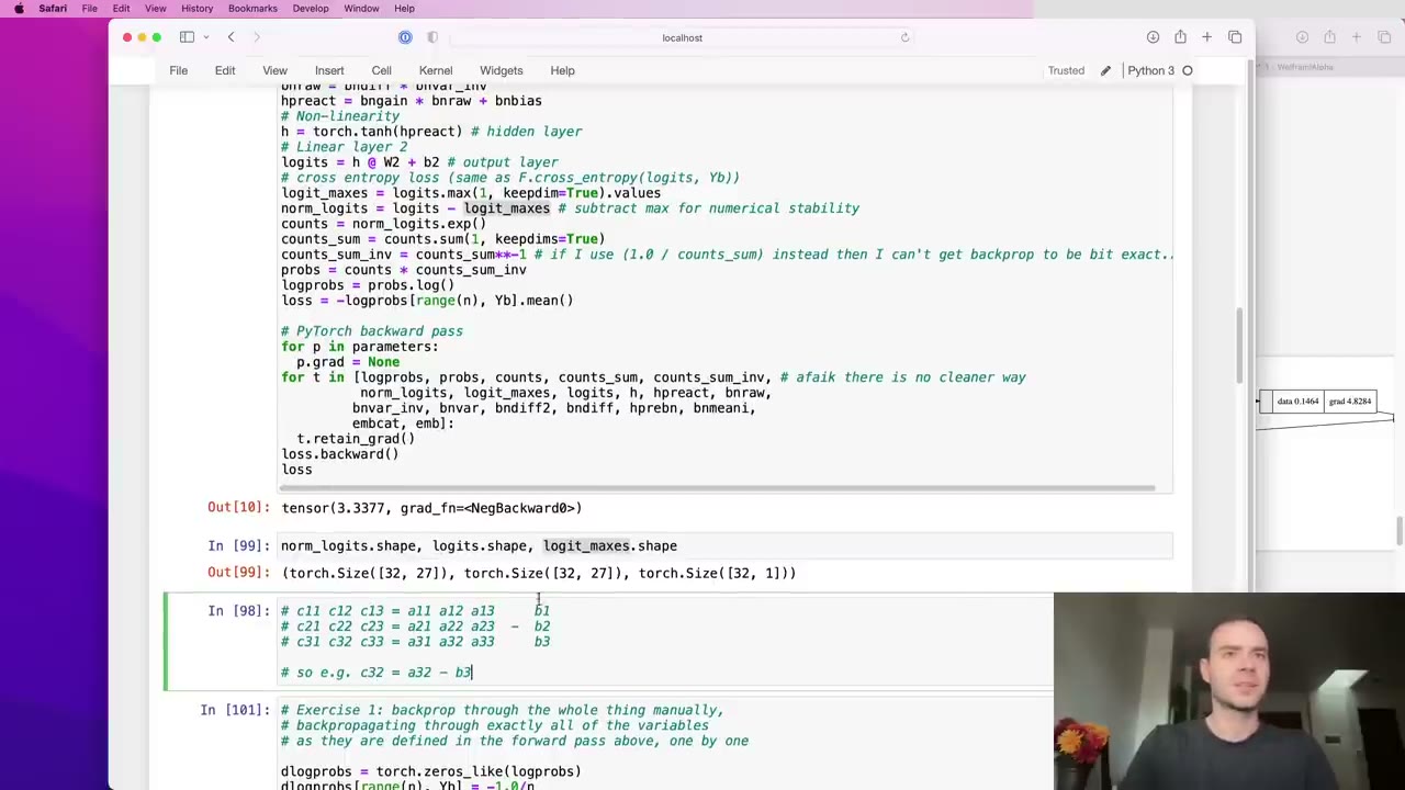
exp is its own derivative, and its output is already stored in counts, so dnorm_logits = counts * dcounts (32:36). The subtraction of logit_maxes broadcasts a column again, so dlogits gets a straight copy of the gradient while dlogit_maxes gets its negative, summed across each row (34:39).
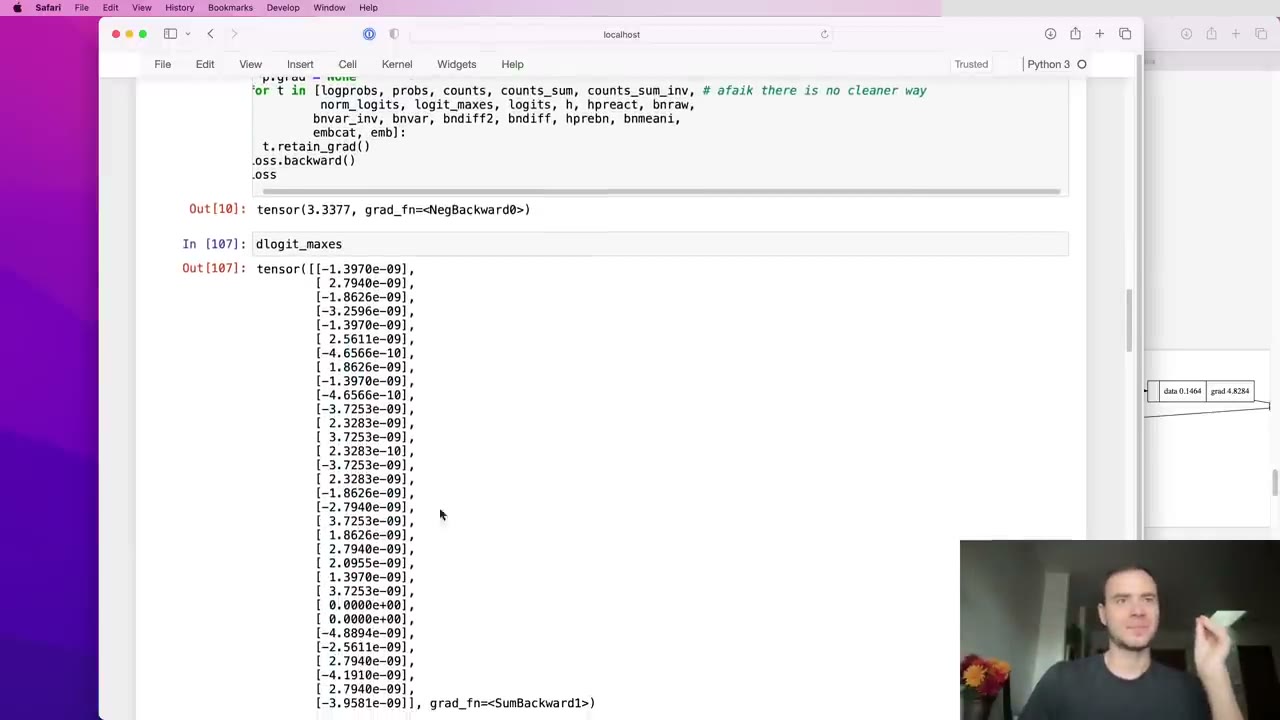
He pauses on that gradient (36:10). Shifting a row of logits by any constant leaves the softmax unchanged, so the maxes cannot affect the loss and their gradient should be zero. It comes out at around 1e-9, which is zero up to floating-point noise. A fused cross-entropy would simply skip this branch; breaking everything into atoms still gets the right answer.
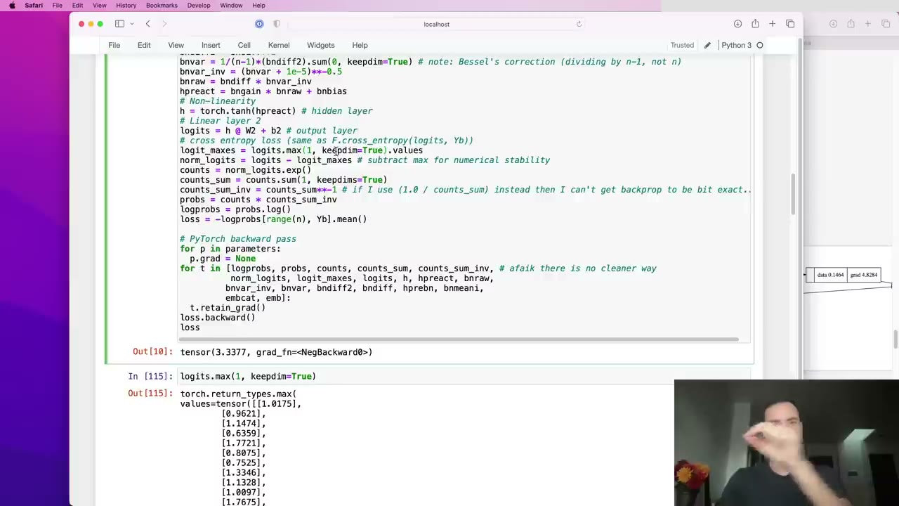
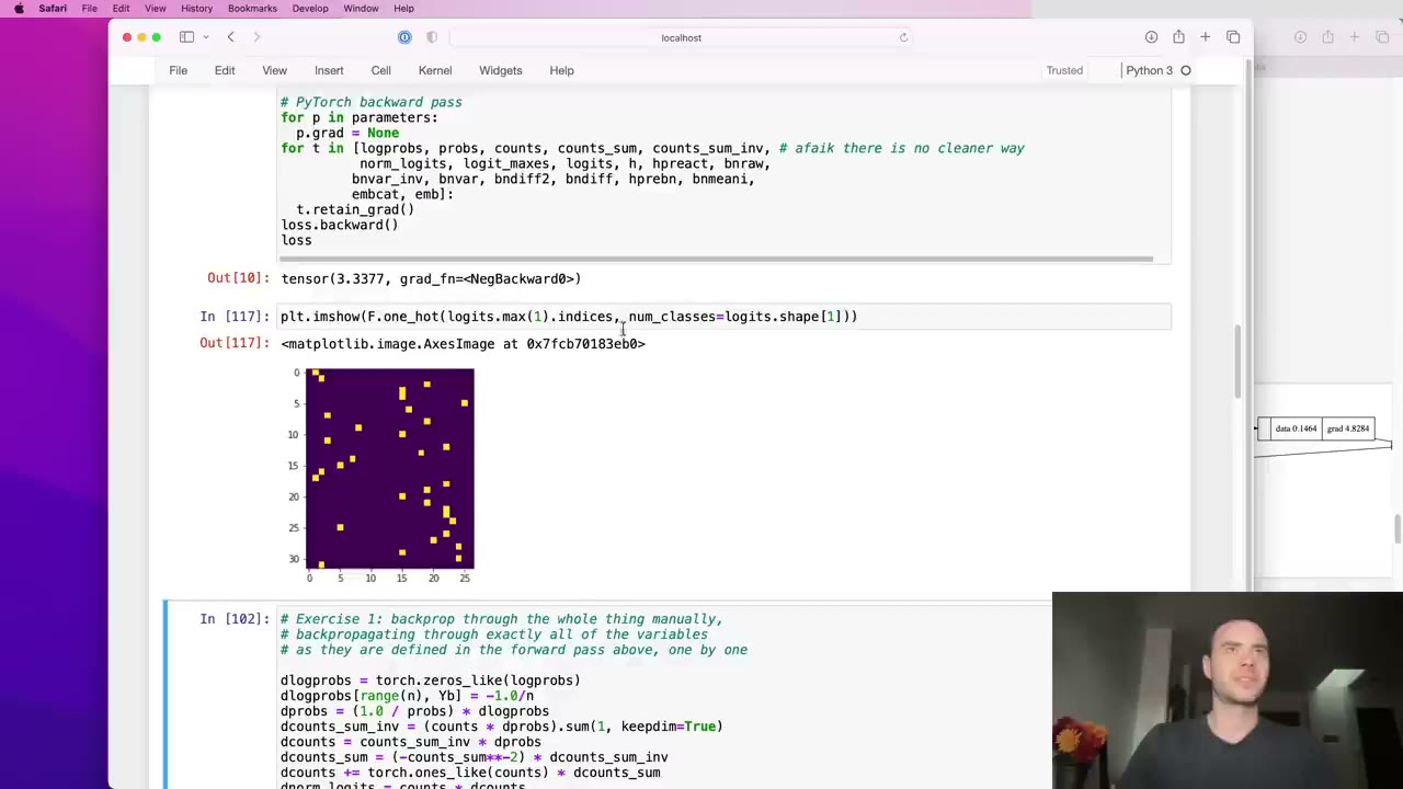
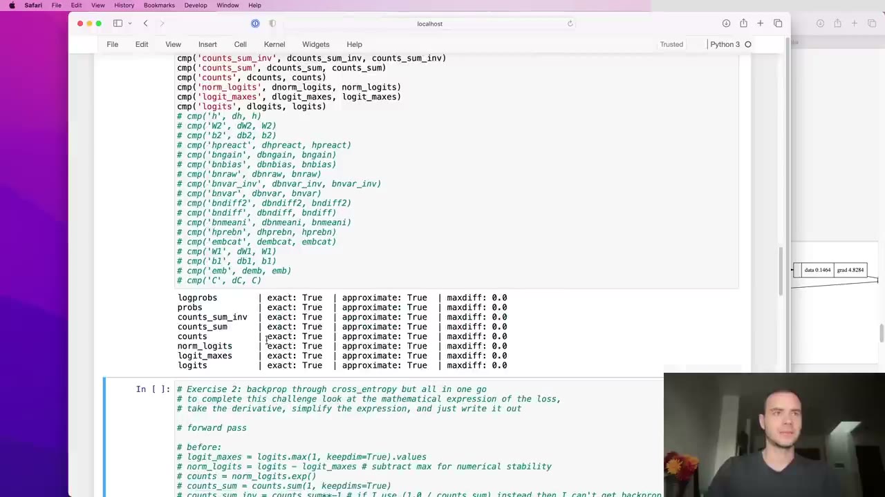
dlogit_maxes is zero up to floating-point noise, as it should be, since the maxes don't change the loss.logits also feeds the max itself, a second branch (38:13). max returns both the values and the indices where they came from, and the gradient should land only at those indices. Instead of building a zero tensor and filling it, he uses F.one_hot on the indices with 27 classes, multiplied by the 32×1 dlogit_maxes so the broadcast routes each value into its row’s one hot position (40:18).
max returns values and indices; the indices say where the gradient should go.
logits matches exactly.41:51 – 53:21 Backprop through a linear layer by matching shapes
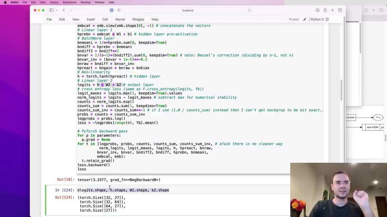
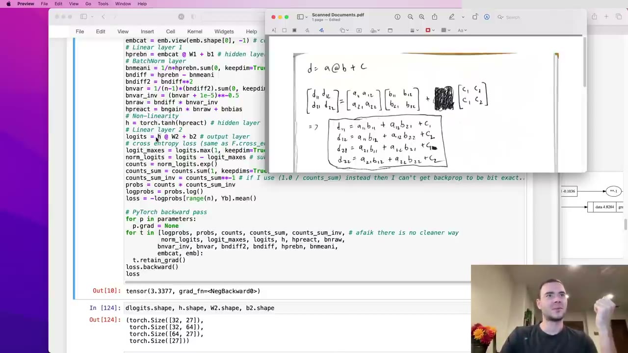
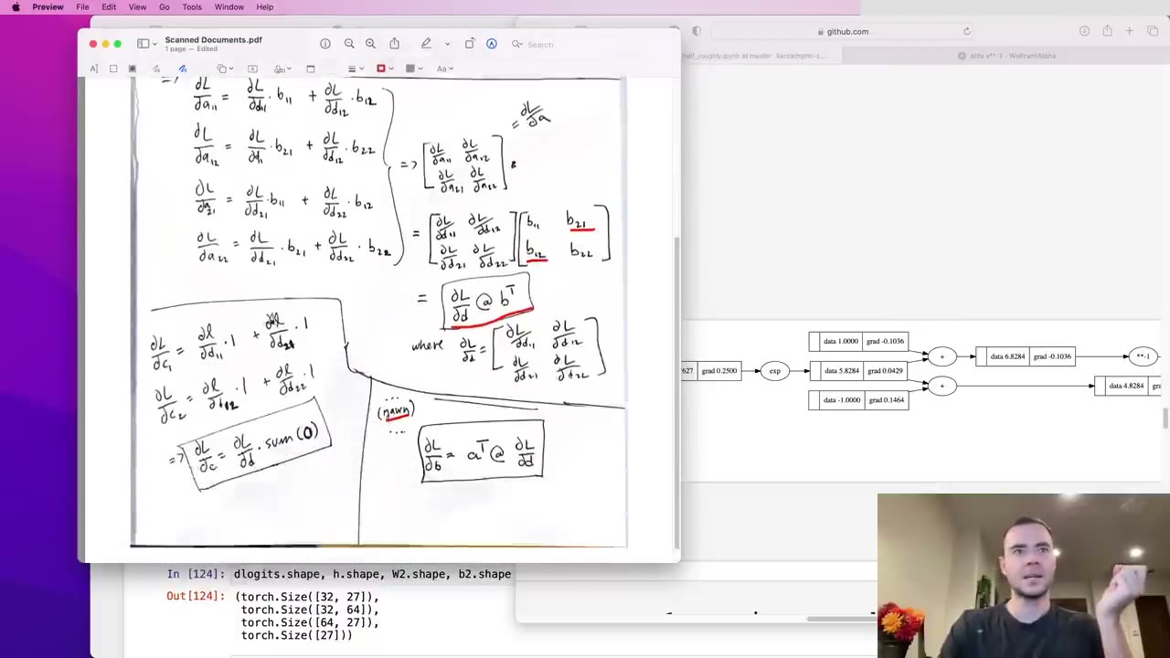
logits = h @ W2 + b2 brings in a matrix multiply plus a 27-element bias that broadcasts down 32 rows. Karpathy refuses to look up matrix calculus. Instead (43:25), he works through d = a @ b + c with 2×2 matrices on paper. Written out, each entry of d is just multiplies and adds, which micrograd already handles. Collecting the derivatives for a turns out to be the incoming gradient multiplied by b transposed (47:03). The gradient for b is a transposed times the incoming gradient, and the bias gets a column sum.
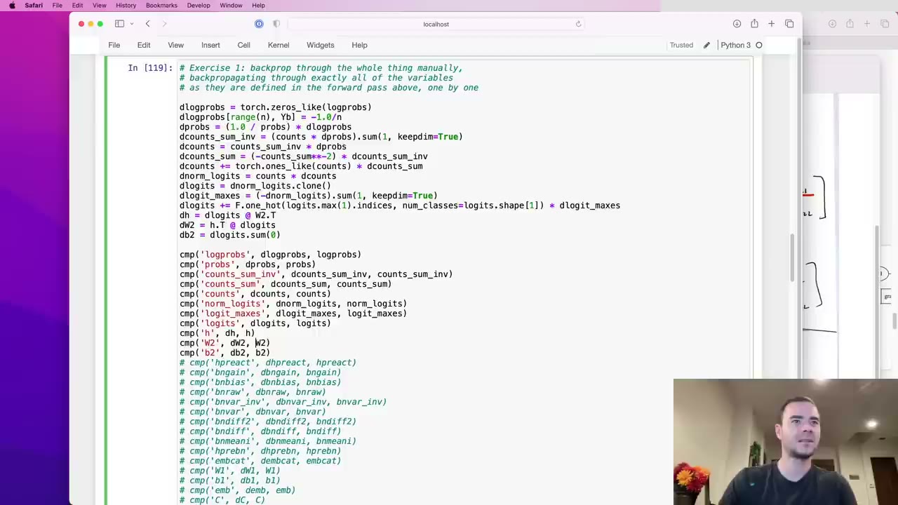
Then the “secret” (49:41): he never remembers these formulas. He knows that dh must be 32×64 and must be some product of dlogits (32×27) and W2 (64×27). Only dlogits @ W2.T fits. The same argument gives h.T @ dlogits for dW2, and db2 must be a sum over dimension 0 because that’s the only way to get 27 numbers out of a 32×27 tensor (52:17). All three match.
53:21 – 59:36 tanh and the BatchNorm gain and bias
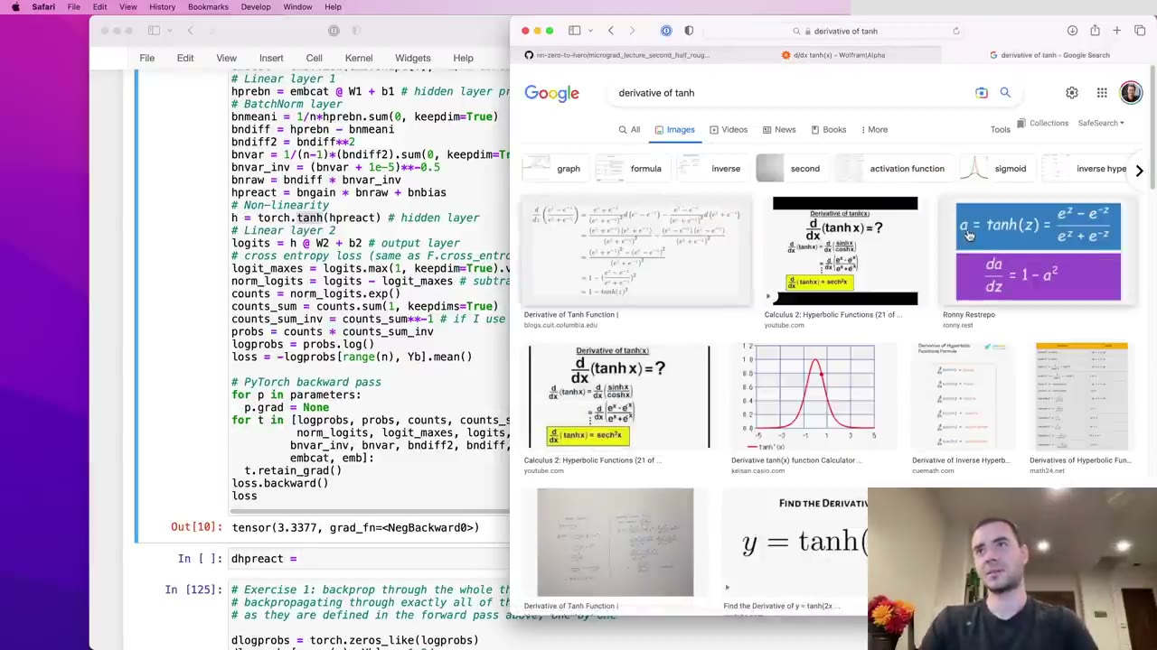
For tanh (53:52), Wolfram Alpha returns a squared hyperbolic secant, which isn’t helpful. The friendlier form is one minus the output squared, and since h is the output, dhpreact = (1 - h**2) * dh.
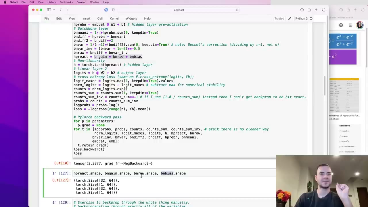
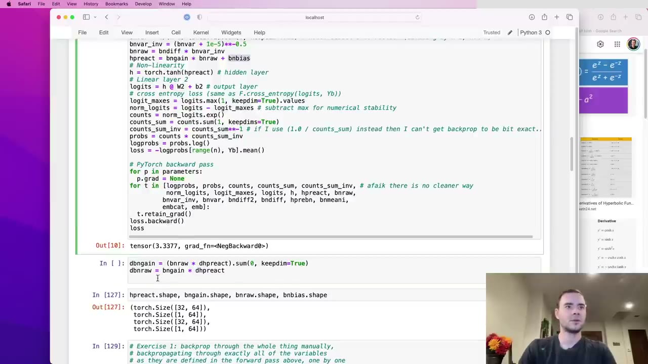
Next is hpreact = bngain * bnraw + bnbias (54:56). This multiply is element-wise, unlike the matrix multiply above, so each factor’s gradient is the other factor times dhpreact. Gain and bias are 1×64 and get replicated down the batch, so their gradients are summed over dimension 0 with keepdim=True. dbnraw needs no sum: the gain broadcasts in the backward pass just as it did in the forward (58:05). He admits he can’t recall why he made gain and bias 2-D while b1 and b2 are 1-D; what matters is being consistent.
dbngain sums over the batch; dbnraw needs no sum.59:36 – 1:05:20 Inside BatchNorm: bnraw and bnvar_inv
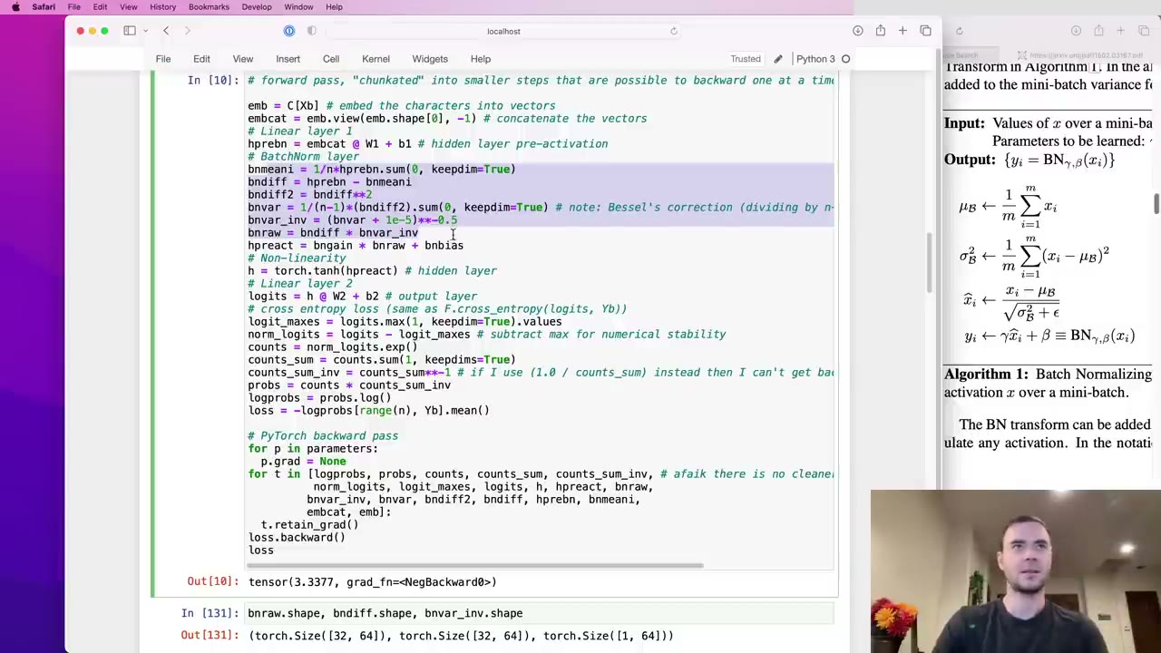
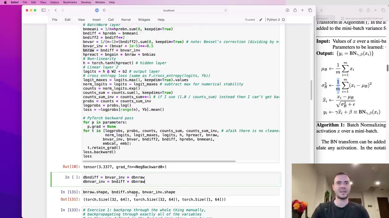
Karpathy maps the split-up BatchNorm onto the paper’s equations (59:36): the mean bnmeani, the centred values bndiff, their squares bndiff2, the variance bnvar, the inverse standard deviation bnvar_inv with epsilon 1e-5, and the normalized output bnraw. He apologises for the variable names.
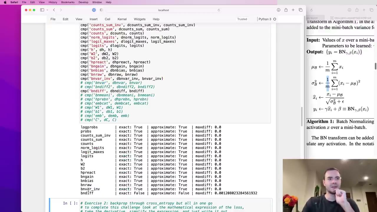
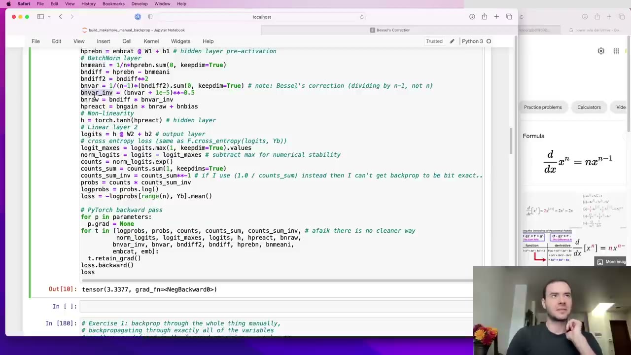
bnraw = bndiff * bnvar_inv gives dbndiff straight away and dbnvar_inv with a sum over the batch (1:01:40). cmp then reports dbndiff as wrong (1:03:16), which is expected because bndiff also feeds the variance branch. He’s glad to see it: the checker can catch a wrong gradient, not just approve correct ones. The power rule gives dbnvar from the **-0.5 (1:04:18).
bnvar_inv is 1×64, so its gradient will need a sum over the batch.
bndiff fails, as expected, because its second branch through the variance isn't in yet.
**-0.5.1:05:20 – 1:09:00 Aside: Bessel’s correction and a train/test mismatch
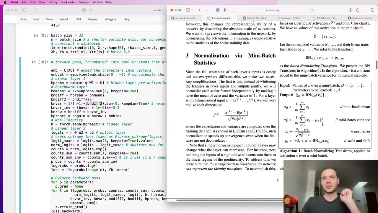
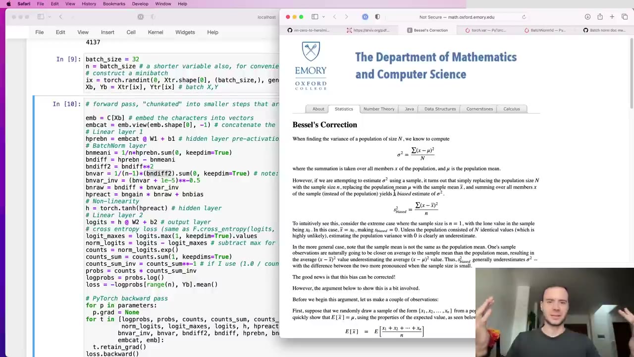
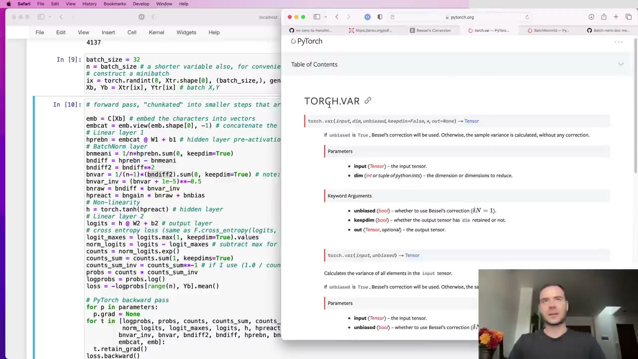
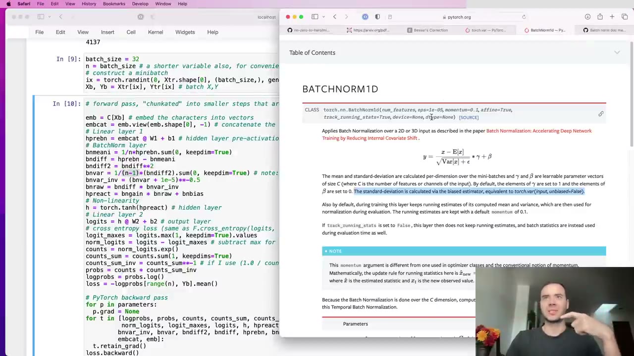
Why 1/(n-1) and not the paper’s 1/m? Dividing by n gives the biased variance estimate, which tends to underestimate the variance of a small sample like a mini-batch; n−1 corrects that (1:06:22). His complaint is that the BatchNorm paper uses the biased version in training and the unbiased one for the inference statistics, and PyTorch’s BatchNorm1d follows it, while its documentation is confusing on the point (1:07:26). He calls the mismatch a bug and uses n−1 in both places, noting that it matters less with bigger batches.
torch.var applies Bessel's correction through its unbiased argument.
Our note: in current PyTorch, torch.var divides by n−1 by default (now expressed as correction=1), and BatchNorm1d still normalizes with the biased variance during training while updating running_var with the unbiased one.
1:09:00 – 1:18:32 Sums become broadcasts: finishing BatchNorm
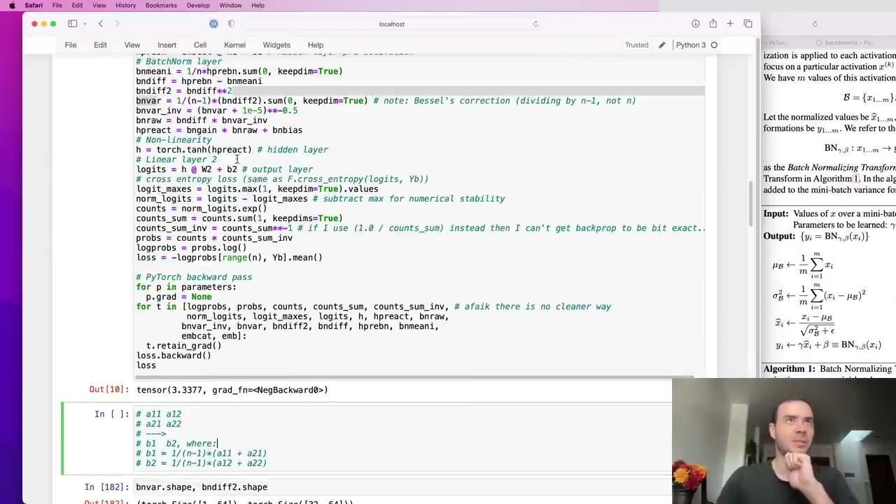
Before working out the variance line, Karpathy states the pattern that has been building up (1:09:32). A sum in the forward pass turns into replication in the backward pass, along the same dimension. Replication in the forward pass means reuse, which turns into a sum. They’re duals.
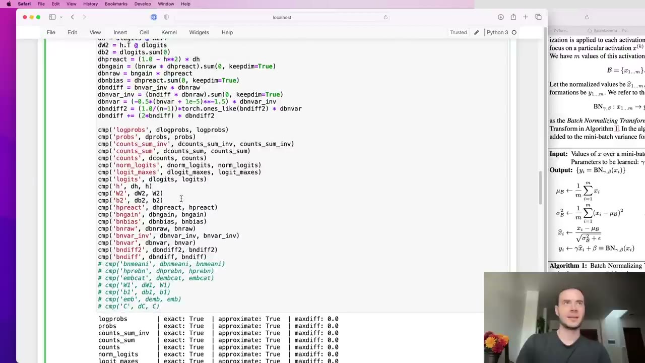
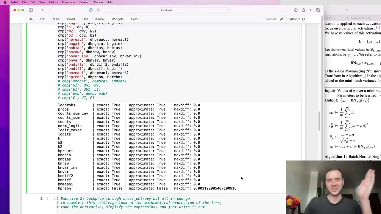
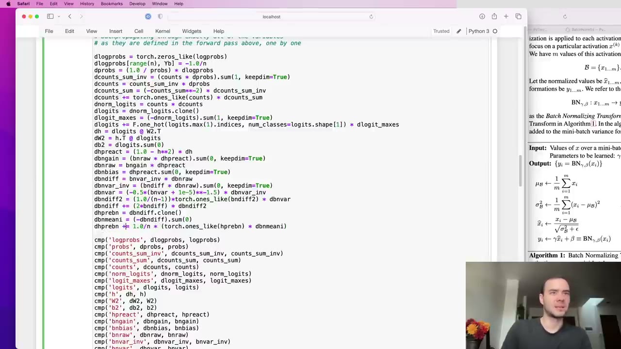
So the variance’s gradient is spread back over all 32 rows, scaled by 1/(n−1), with torch.ones_like and broadcasting doing the copying (1:11:37). Squaring gives a local derivative of 2 * bndiff, and adding it to the earlier branch makes dbndiff correct at last (1:13:42). The mean subtraction mirrors the logit_maxes case: dhprebn starts as a copy, dbnmeani is the negated sum over the batch, and cmp again flags dhprebn as incomplete (1:16:22). The mean’s own backward pass, scaled by 1/n and broadcast over the rows, supplies the missing piece (1:16:53).
dbndiff2, then the second contribution to dbndiff added with +=.
hprebn is still incomplete: the branch through the mean is missing.
+= lines in place.1:18:32 – 1:26:25 First layer, view, and the embedding lookup
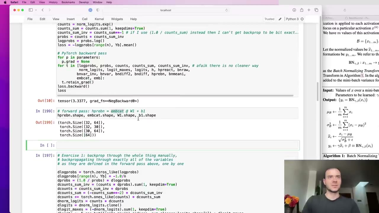
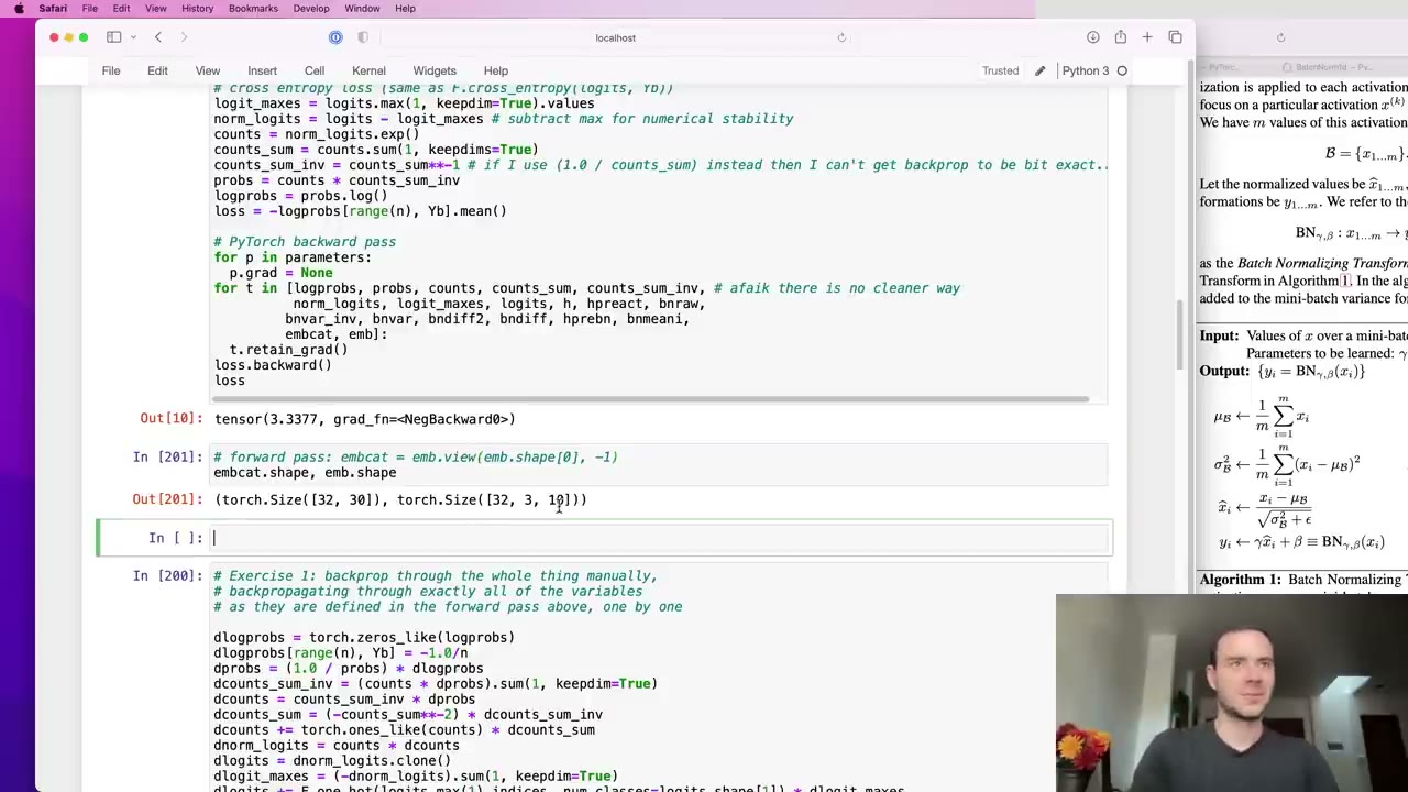
The first linear layer falls to shape matching again (1:19:04): embcat is 32×30, W1 is 30×64, and b1 is a plain 64-vector, so its sum over dimension 0 drops the kept dimension. Undoing the concatenation is trivial (1:21:08): view only reinterprets memory, so the gradient is viewed back to the 32×3×10 shape of emb.
b1 is a plain 64-vector.
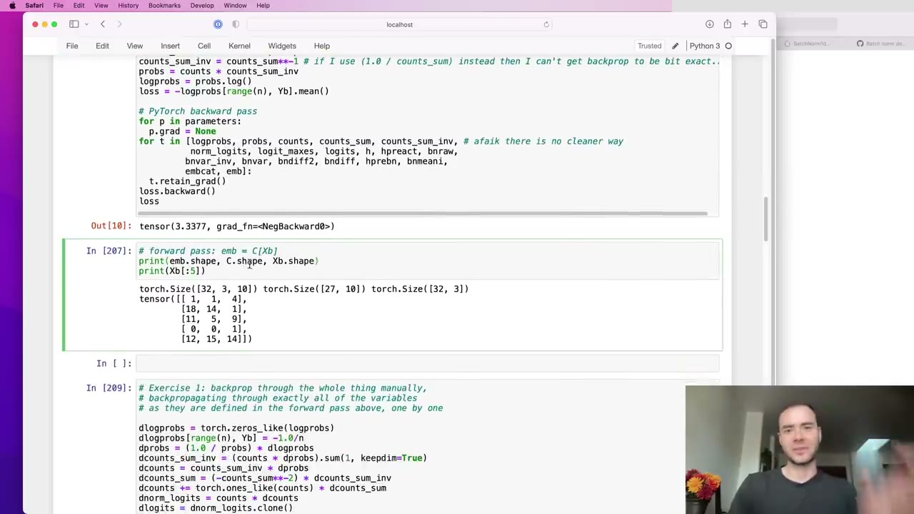
view turned 32×3×10 into 32×30, so the gradient is viewed back.The last step reverses C[Xb] (1:22:11). Every entry of Xb named a row of the 27×10 table C, and that row was copied into one slot of emb. Going backwards, each slot’s 10-number gradient goes back to its row of dC, adding whenever a character appears more than once in the batch, which it almost always does. He writes it as a double for loop and invites a vectorized version (1:24:15). Every gradient now matches.
Xb picks a row of the 27×10 table C.
Our note: one vectorized form is dC.index_add_(0, Xb.view(-1), demb.view(-1, 10)), which accumulates repeated indices the same way the loop does.
1:26:25 – 1:32:37 Exercise 2: cross-entropy in one step
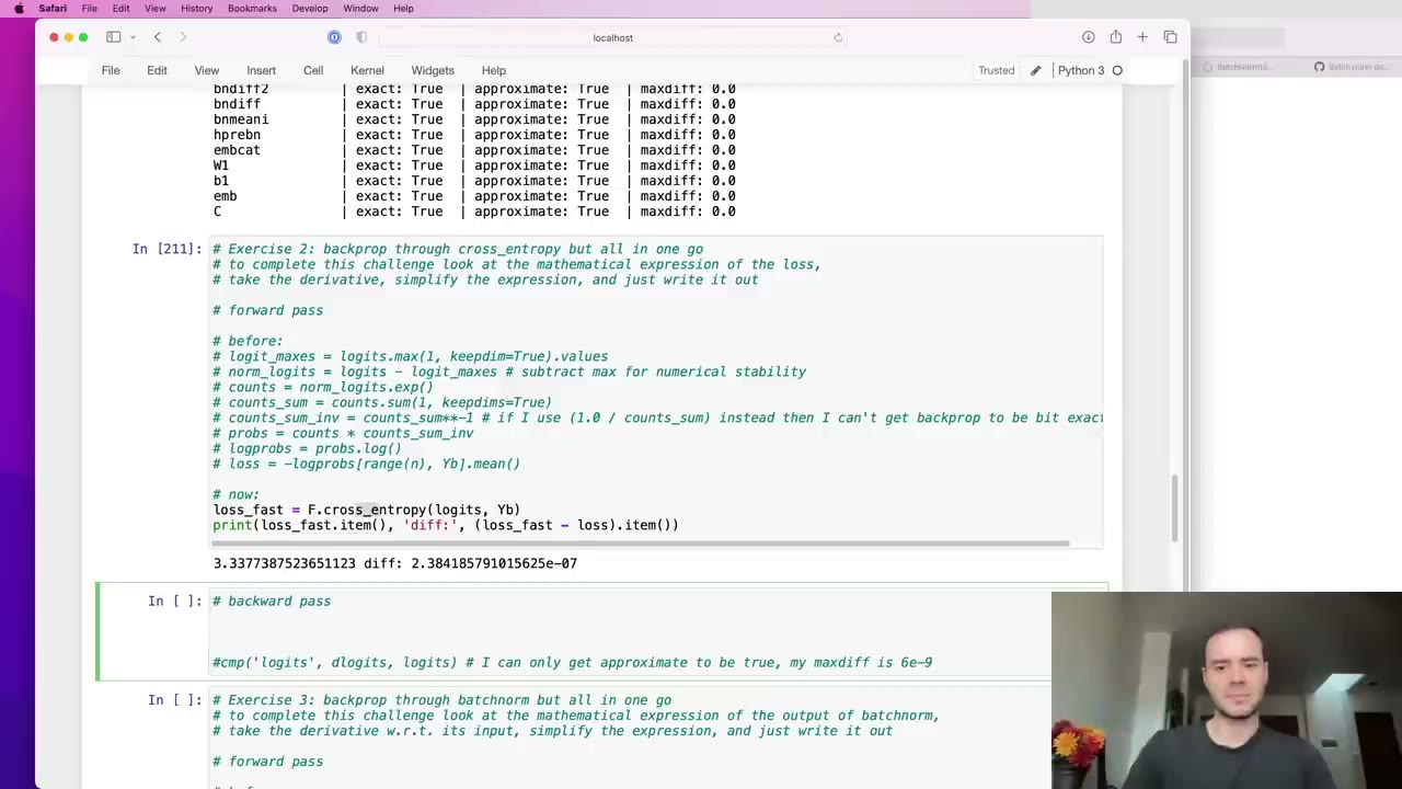
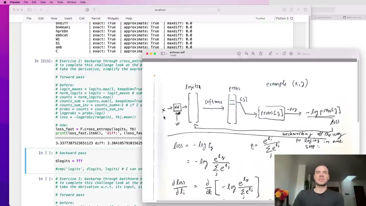
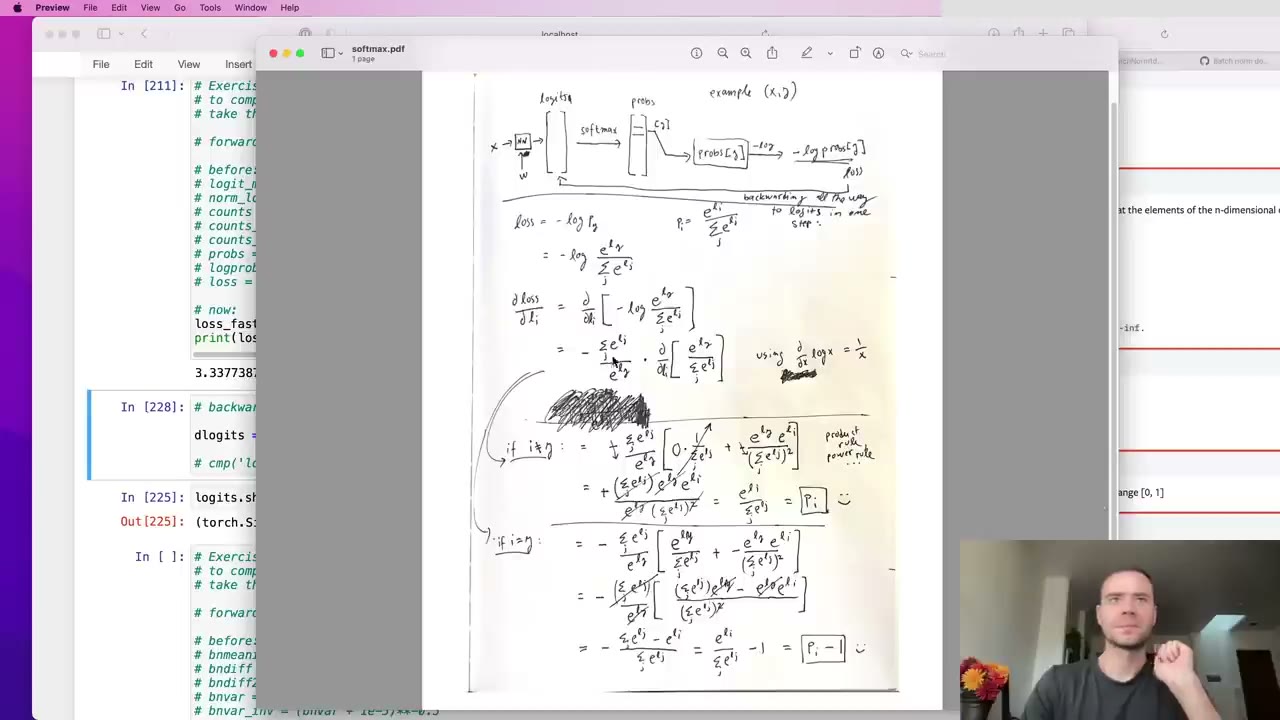
Exercise 1 did far more work than necessary (1:26:25). Written as one formula, the loss is the negative log of the softmax probability at the correct label, averaged over the batch, and differentiating that on paper makes most terms cancel. F.cross_entropy gives the same loss and is faster in both directions.
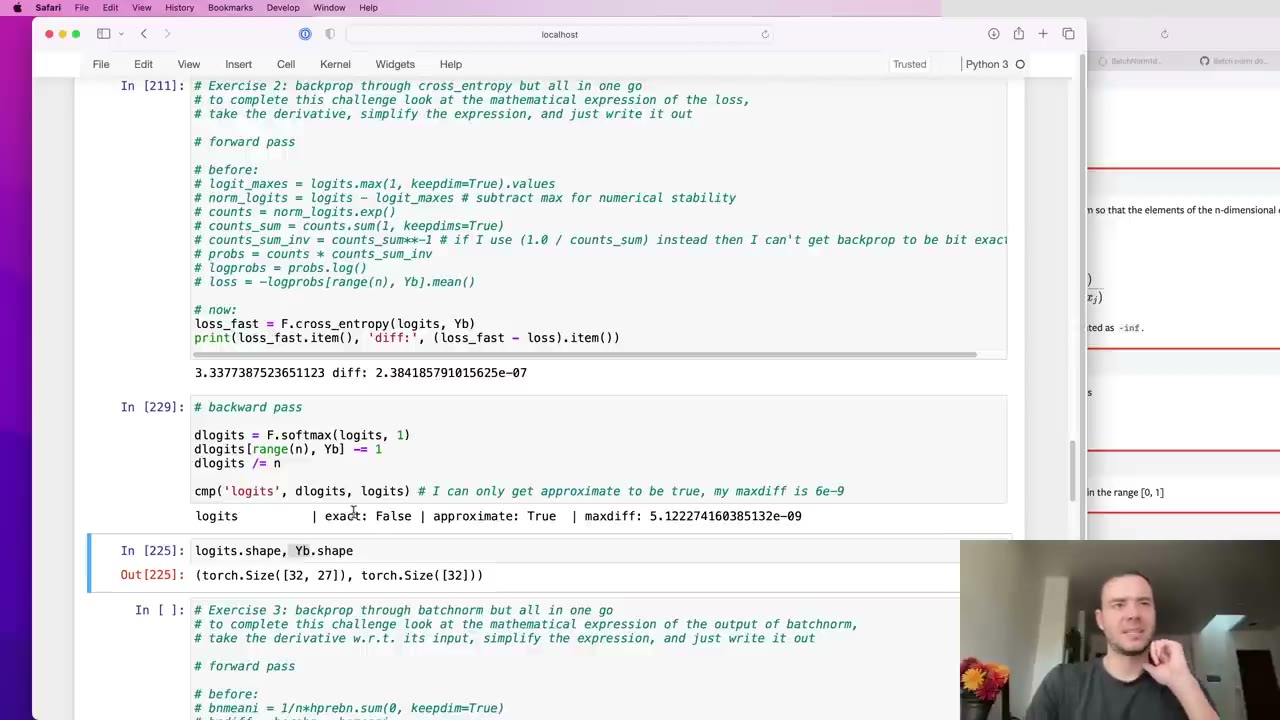
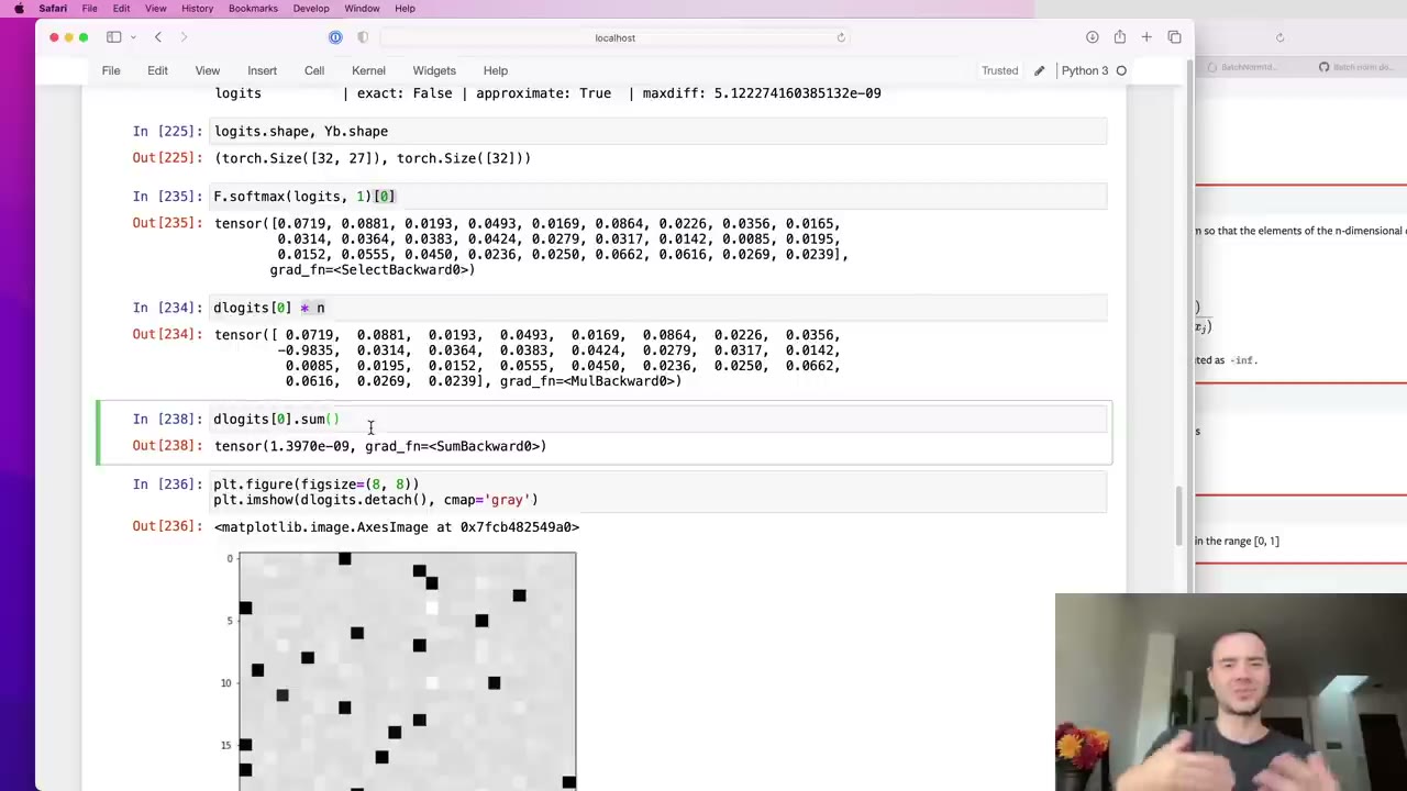
F.cross_entropy gives the same loss as the long version, to within about 2e-7.He sets it up as a pen-and-paper problem (1:28:29), then shows the result (1:30:02). Split the derivative into two cases, the logit at the label and every other logit, and you get the softmax probability, minus 1 at the label. Divide by n for the batch mean and it’s three lines of code. The match is approximate, with a maximum difference around 5e-9 from floating-point differences (1:32:05).
1:32:37 – 1:36:41 Gradients as push and pull
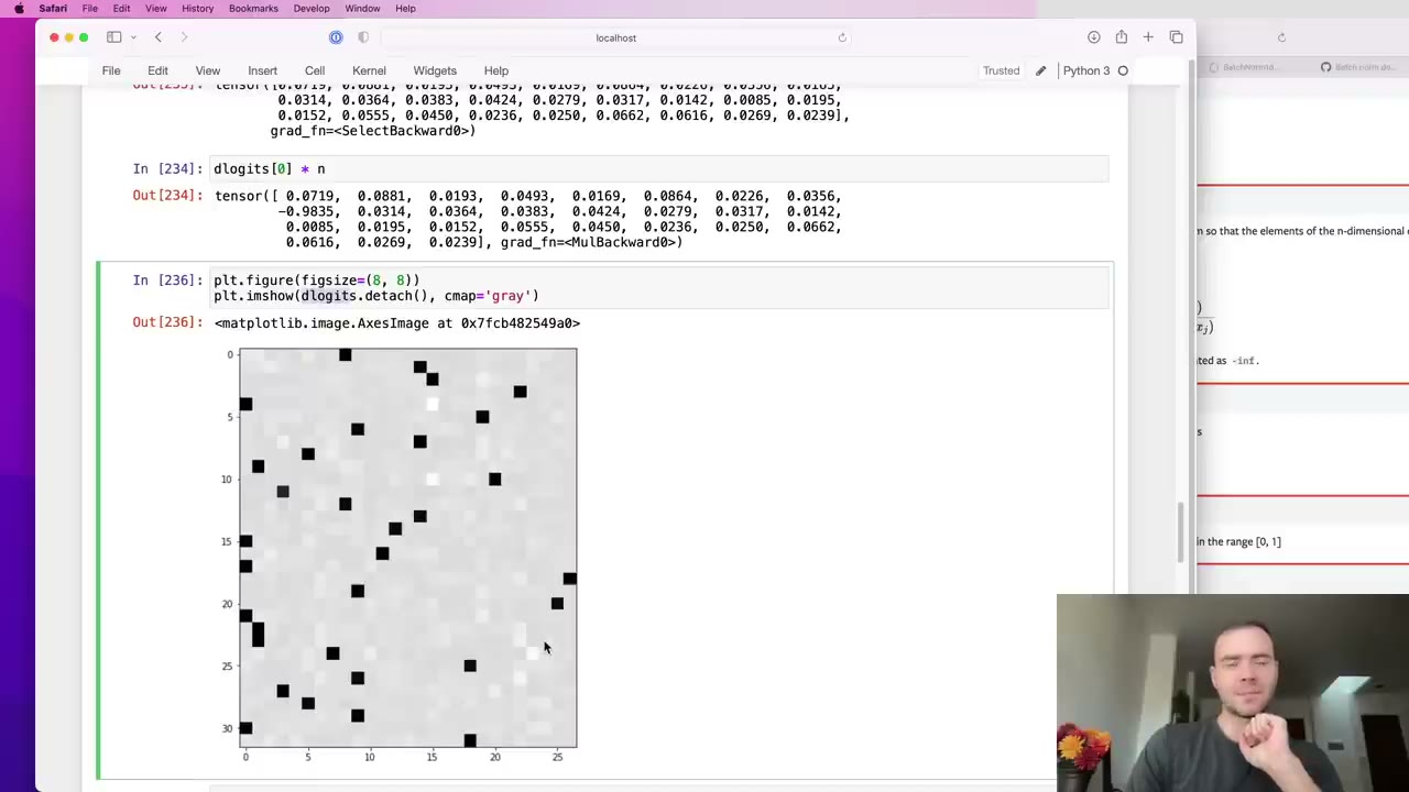
This is the lecture’s best piece of intuition. Plotting dlogits (1:32:37) shows the probability matrix with dark cells at the correct characters. Each row sums to zero. Karpathy reads it as forces (1:34:08): the wrong characters are pulled down in proportion to the probability they got, the right one is pulled up by an equal total amount, and the network is a big pulley system that passes those tugs back to the weights. A perfect prediction produces a row of zeros: no pull at all (1:35:39). A confident mistake produces a strong pull on that one wrong character.
dlogits as an image: the black cells are the correct characters being pulled up.
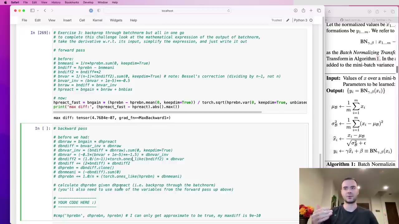
1:36:41 – 1:43:57 Exercise 3: BatchNorm backward on paper
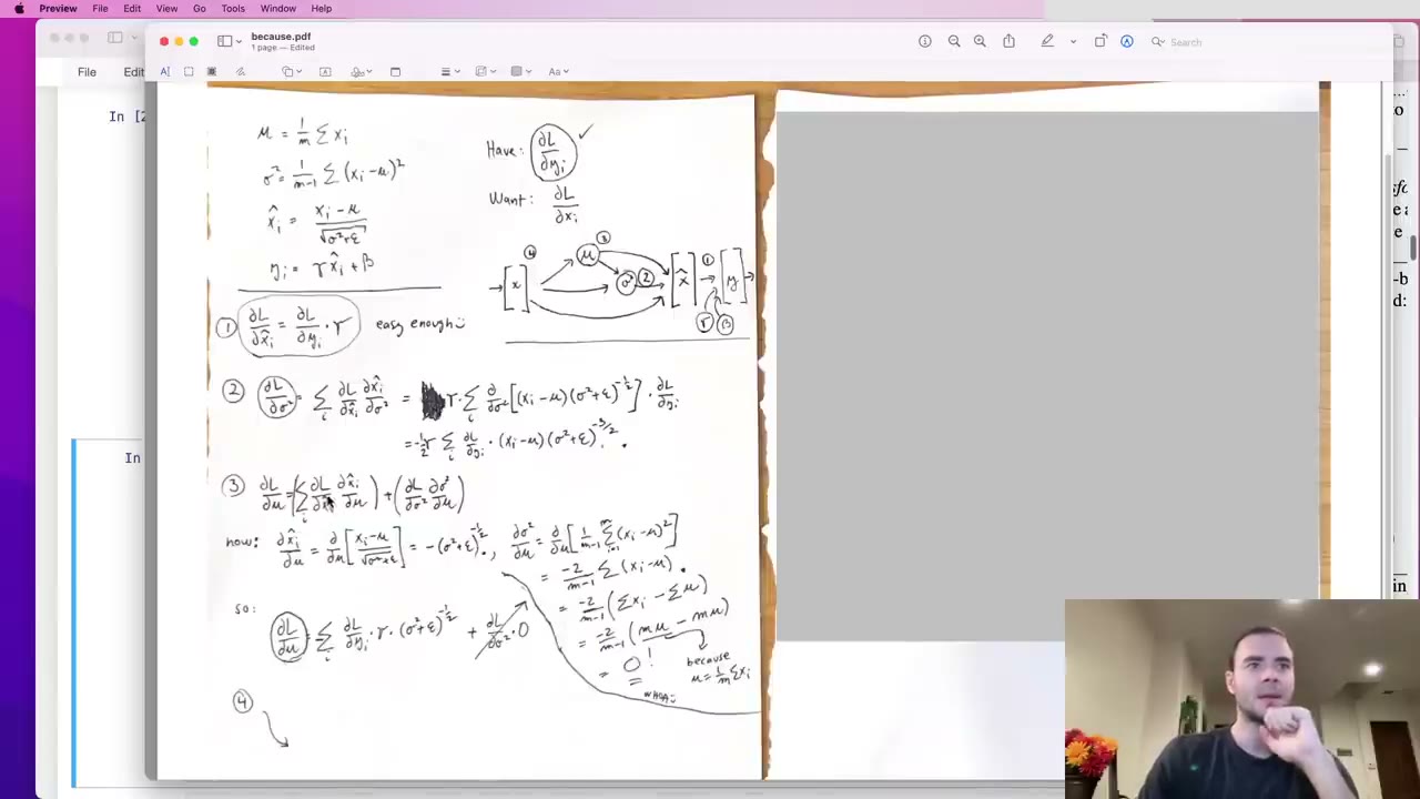
Exercise 3 does the same for BatchNorm (1:36:41): glue it into one expression and derive dhprebn from dhpreact directly, ignoring gain and bias since their gradients are easy. He writes the paper’s equations with Bessel’s correction and suggests an order: x̂, then σ², then μ, then x, like a topological sort done in symbols (1:39:15).
dhprebn.
The warning he repeats is that x, x̂ and y are vectors of 32 numbers, while μ and σ² are single numbers. Draw it wrong and the math goes wrong. σ² fans out into all 32 x̂ values, so its gradient is a sum over i (1:40:48). μ has 33 outgoing arrows, 32 to the x̂ values and one to σ² (1:41:51). A nice cancellation appears: because μ is exactly the mean of the x values, the derivative of σ² with respect to μ is zero, so that whole term drops out (1:42:54).
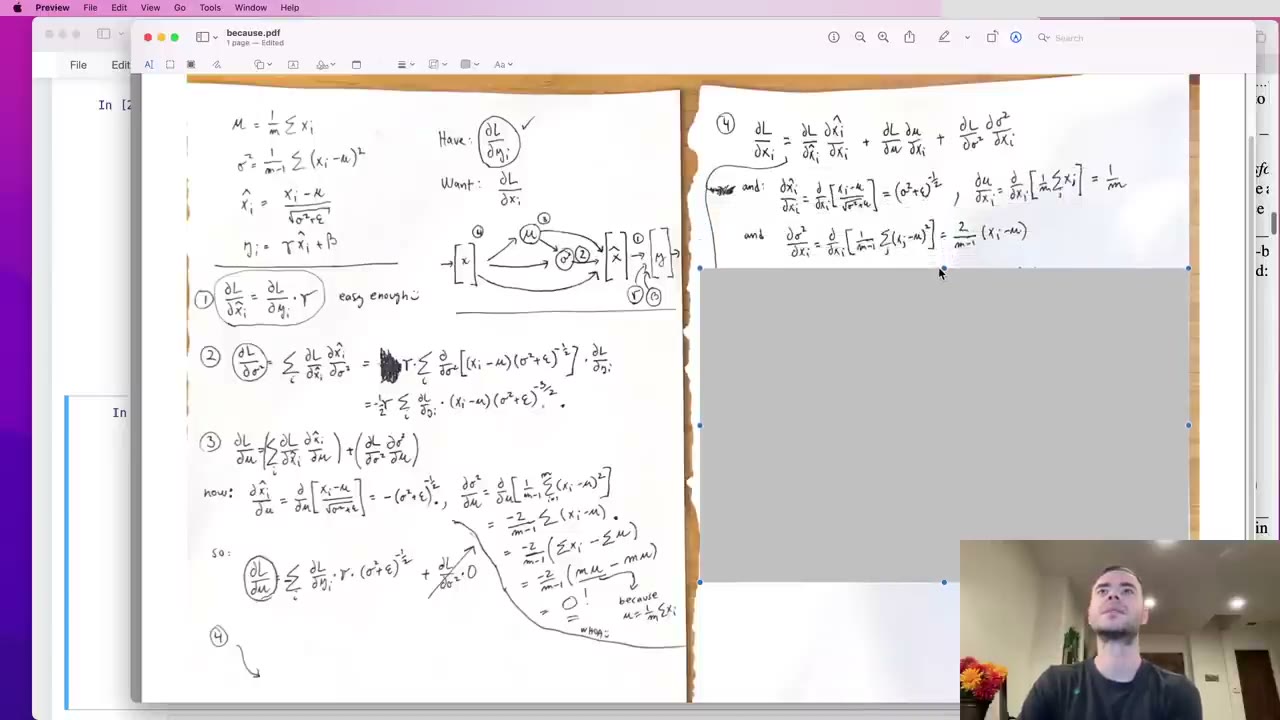
1:43:57 – 1:50:13 The gradient for x, and one line of code
Each input xᵢ reaches the loss three ways: through μ, through σ², and through its own x̂ᵢ (1:43:57). The chain rule adds the three. The fiddly part is substitution (1:46:01): the sums inside the σ² and μ gradients use their own loop index, so it has to be renamed to j before plugging in, or the result mixes up the particular xᵢ with the terms being summed. Splitting the (σ²+ε)^(−3/2) factor into three copies of (σ²+ε)^(−1/2) lets the expression fold back into x̂ terms (1:47:04).
The final line of code matches PyTorch to a tiny difference (1:48:38). He stresses that getting from the paper formula to working code is an exercise in itself: the derivation is for one neuron over 32 examples, while the code must run all 64 neurons in parallel and broadcast every sum correctly.
1:50:13 – end Exercise 4: training without loss.backward()
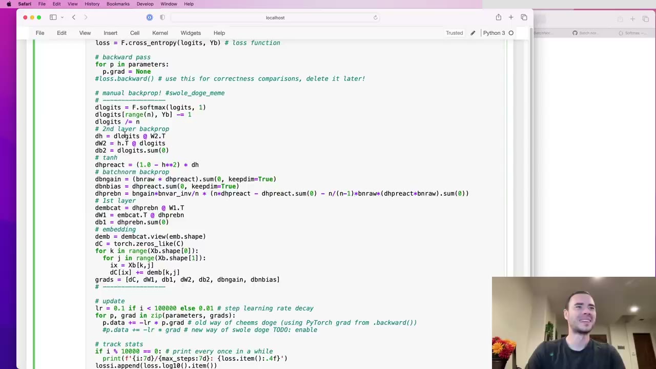
The final exercise rebuilds the network from scratch and pastes in all the manual pieces, using the fast cross-entropy and BatchNorm versions (1:50:13). The whole backward pass is about 20 lines. A first run of 100 steps stops to compare against PyTorch: approximately equal, with tiny differences (roughly 1e-9 to 1e-8 on screen) whose source he isn’t sure of (1:51:15). Then loss.backward() is commented out (“it feels amazing to say that”), the update zips parameters with the hand-computed gradients instead of reading p.grad, and the loop is wrapped in torch.no_grad() so PyTorch skips building a graph (1:52:16).
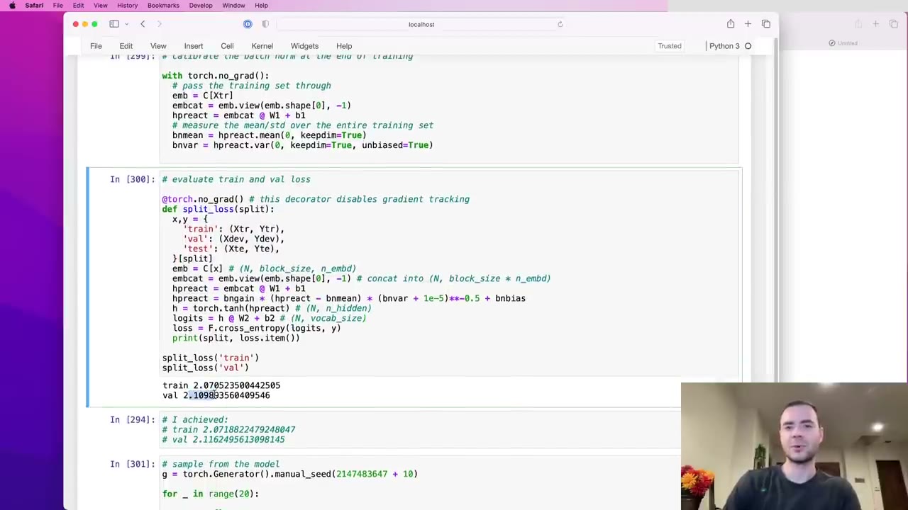
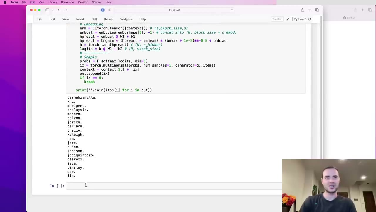
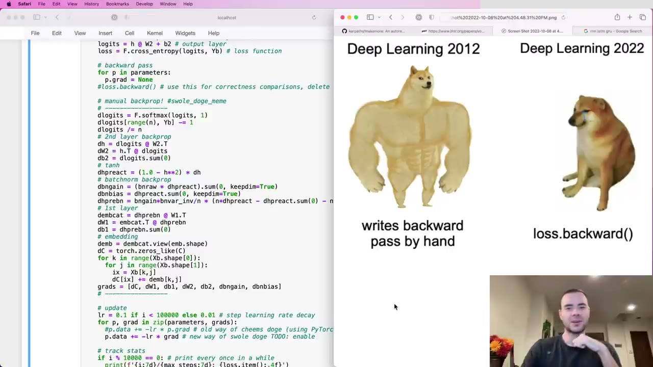
loss.backward() commented out and the update using the hand-computed gradients.After training and a separate pass to calibrate the BatchNorm statistics, the loss is close to earlier lectures and the samples are the same kind of name-like strings (1:53:20). Karpathy’s verdict: each layer’s backward is a few lines, with BatchNorm the exception. In practice you’d still use autograd, but now you know what it does. Next up, he says, are recurrent networks and LSTMs (1:54:55).
Our note: the next lecture on the playlist turned out to be the WaveNet-style model of Lecture 6 instead. Recurrent networks never got their own lecture.
Code you’ll write
These excerpts follow the lecture notebook; the full starter and solution code is in the MIT-licensed nn-zero-to-hero repository (lectures/makemore), and the standalone model code lives in makemore. Variables: n is the batch size (32), Xb, Yb the batch inputs and labels.
Backprop through the chunked cross-entropy (12:55). Every line undoes one forward line, with += where a tensor feeds two branches.
dlogprobs = torch.zeros_like(logprobs)
dlogprobs[range(n), Yb] = -1.0/n
dprobs = (1.0 / probs) * dlogprobs
dcounts_sum_inv = (counts * dprobs).sum(1, keepdim=True)
dcounts = counts_sum_inv * dprobs
dcounts_sum = (-counts_sum**-2) * dcounts_sum_inv
dcounts += torch.ones_like(counts) * dcounts_sum
dnorm_logits = counts * dcounts
dlogits = dnorm_logits.clone()
dlogit_maxes = (-dnorm_logits).sum(1, keepdim=True)
dlogits += F.one_hot(logits.max(1).indices, num_classes=logits.shape[1]) * dlogit_maxes
Second linear layer, tanh, and BatchNorm’s scale and shift (50:11). Matrix multiplies come from matching shapes; broadcast parameters get summed over the batch.
dh = dlogits @ W2.T
dW2 = h.T @ dlogits
db2 = dlogits.sum(0)
dhpreact = (1.0 - h**2) * dh
dbngain = (bnraw * dhpreact).sum(0, keepdim=True)
dbnraw = bngain * dhpreact
dbnbias = dhpreact.sum(0, keepdim=True)
Through BatchNorm’s internals, one line at a time (1:01:40). Note the n−1 from Bessel’s correction and the two += lines that complete branches.
dbndiff = bnvar_inv * dbnraw
dbnvar_inv = (bndiff * dbnraw).sum(0, keepdim=True)
dbnvar = (-0.5 * (bnvar + 1e-5)**-1.5) * dbnvar_inv
dbndiff2 = (1.0/(n-1)) * torch.ones_like(bndiff2) * dbnvar
dbndiff += (2 * bndiff) * dbndiff2
dhprebn = dbndiff.clone()
dbnmeani = (-dbndiff).sum(0)
dhprebn += 1.0/n * (torch.ones_like(hprebn) * dbnmeani)
First layer and the embedding table (1:19:04). view is undone by viewing back; indexing is undone by scattering and adding.
dembcat = dhprebn @ W1.T
dW1 = embcat.T @ dhprebn
db1 = dhprebn.sum(0)
demb = dembcat.view(emb.shape)
dC = torch.zeros_like(C)
for k in range(Xb.shape[0]):
    for j in range(Xb.shape[1]):
        ix = Xb[k, j]
        dC[ix] += demb[k, j]
Exercise 2: the cross-entropy gradient in one go (1:31:04). Softmax minus one-hot, divided by the batch size.
dlogits = F.softmax(logits, 1)
dlogits[range(n), Yb] -= 1
dlogits /= n
Exercise 3: the BatchNorm backward pass as a single expression (1:48:38). It reuses bnraw (x̂) and bnvar_inv from the forward pass and runs for all 64 neurons at once.
dhprebn = bngain * bnvar_inv / n * (
    n * dhpreact
    - dhpreact.sum(0)
    - n / (n - 1) * bnraw * (dhpreact * bnraw).sum(0)
)
Skip list
- 3:40 – 7:15 The history tour of hand-written backward passes (Matlab RBMs, 2014 NumPy code). Interesting context, no technique you need.
- 12:23 – 12:55 The suggestion to try the exercises in Colab first. Useful advice, but you only need to hear it once.
- 1:05:20 – 1:09:00 The Bessel’s correction aside. Worth one watch if you implement BatchNorm; skip it on a re-watch that’s only about backprop.
- 1:43:57 – 1:48:38 The full algebra for the BatchNorm input gradient. If you only want the result, jump to 1:48:38 and read the one-line formula; come back when you want to rederive it.
- 1:53:20 – end The trained model’s loss and samples, already familiar from Lecture 4, and the sign-off.
Glossary
- Leaky abstraction — Karpathy’s term for backprop: a tool that mostly hides its internals but breaks in ways you can only fix if you understand them.
cmp— the notebook’s checker that compares a hand-derived gradient with PyTorch’s.gradfor exact and approximate equality and reports the largest difference.- Local derivative — the derivative of one operation’s output with respect to its input, multiplied by the incoming gradient in the chain rule.
- Broadcasting — PyTorch’s automatic replication of a smaller tensor (a 32×1 column, a 1×64 row) to match a larger one. In the backward pass, a broadcast becomes a sum along the same dimension.
- Gradient accumulation across branches — when one tensor is used in several places, its total gradient is the sum of the gradients from each use, hence
+=. - Shape matching — deriving matrix-multiply gradients by asking which product of the incoming gradient and the other factor, with which transpose, gives the right shape.
- Logits — the raw output scores of the network, one per possible next character, before softmax.
- Softmax — exponentiating logits and normalizing each row so it sums to one; subtracting the row maximum first keeps the exponentials from overflowing without changing the result.
- Cross-entropy loss — the average negative log probability the model assigns to the correct next character. Its gradient with respect to the logits is softmax minus one-hot, divided by n.
- BatchNorm — a layer that standardizes each neuron’s pre-activations across the batch, then applies a learned gain and bias.
- Bessel’s correction — dividing a sample’s sum of squared deviations by n−1 instead of n, giving an unbiased variance estimate.
- Train/test mismatch — computing something differently during training and inference; here, the biased vs. unbiased BatchNorm variance.
- Embedding table (
C) — the 27×10 matrix of learned character vectors; its gradient is assembled by routing each slot’s gradient back to the row it came from. torch.no_grad()— a context that tells PyTorch not to record operations for autograd, used once the gradients are computed by hand.
FAQ
Why does Karpathy write the backward pass by hand when PyTorch can do it?
Not because you should in practice. He calls backpropagation a leaky abstraction: you can stack differentiable pieces and still get a network that trains badly or not at all, and you can only debug that if you know how gradients move through each operation. His example is code that clips the loss instead of the gradients, which quietly zeroes the gradient of outliers. Ten years earlier, he adds, writing the backward pass by hand was simply normal.
What is the gradient of the cross-entropy loss with respect to the logits?
For each example, take the softmax probabilities and subtract 1 at the position of the correct character. Because the loss is a mean over the batch, divide the whole thing by the batch size n. In code that is three lines: softmax of the logits along dimension 1, subtract 1 at [range(n), Yb], then divide by n. Each row of the result sums to zero.
Why does the BatchNorm in this lecture divide the variance by n-1?
That is Bessel's correction, which gives an unbiased estimate of the variance from a small sample such as a mini-batch. Karpathy points out that the BatchNorm paper, and PyTorch's BatchNorm1d, use the biased 1/n version during training but the unbiased version for the running statistics used at test time. He considers that train/test mismatch a bug and uses n-1 in both places.
How do you backpropagate through a matrix multiplication without memorizing formulas?
Use the shapes. The gradient of a tensor always has that tensor's shape, and the backward pass of a matrix multiply is another matrix multiply between the incoming gradient and the other factor. Usually only one arrangement, with one transpose, produces the right shape. For logits = h @ W2 + b2 that gives dh = dlogits @ W2.T, dW2 = h.T @ dlogits, and db2 = dlogits.sum(0).
Where is the notebook for Becoming a Backprop Ninja?
In Karpathy's nn-zero-to-hero repository on GitHub, in the lectures/makemore folder, as makemore_part4_backprop.ipynb. The video description also links a Google Colab copy. Karpathy suggests attempting each gradient yourself before watching him give the answer.
Studying another course? Paste its YouTube or Bilibili link on the home page to request a handout — or make your own with the desktop app (coming soon).