Karpathy's Zero to Hero, Lecture 7: Let's build GPT — notes, code and timestamps

Updated 2026-10-07 · Video: Andrej Karpathy, published 2023-01-17 · 116 min

77 key slides

0:362:223:545:006:258:058:4010:0311:3111:4113:2513:4616:0317:11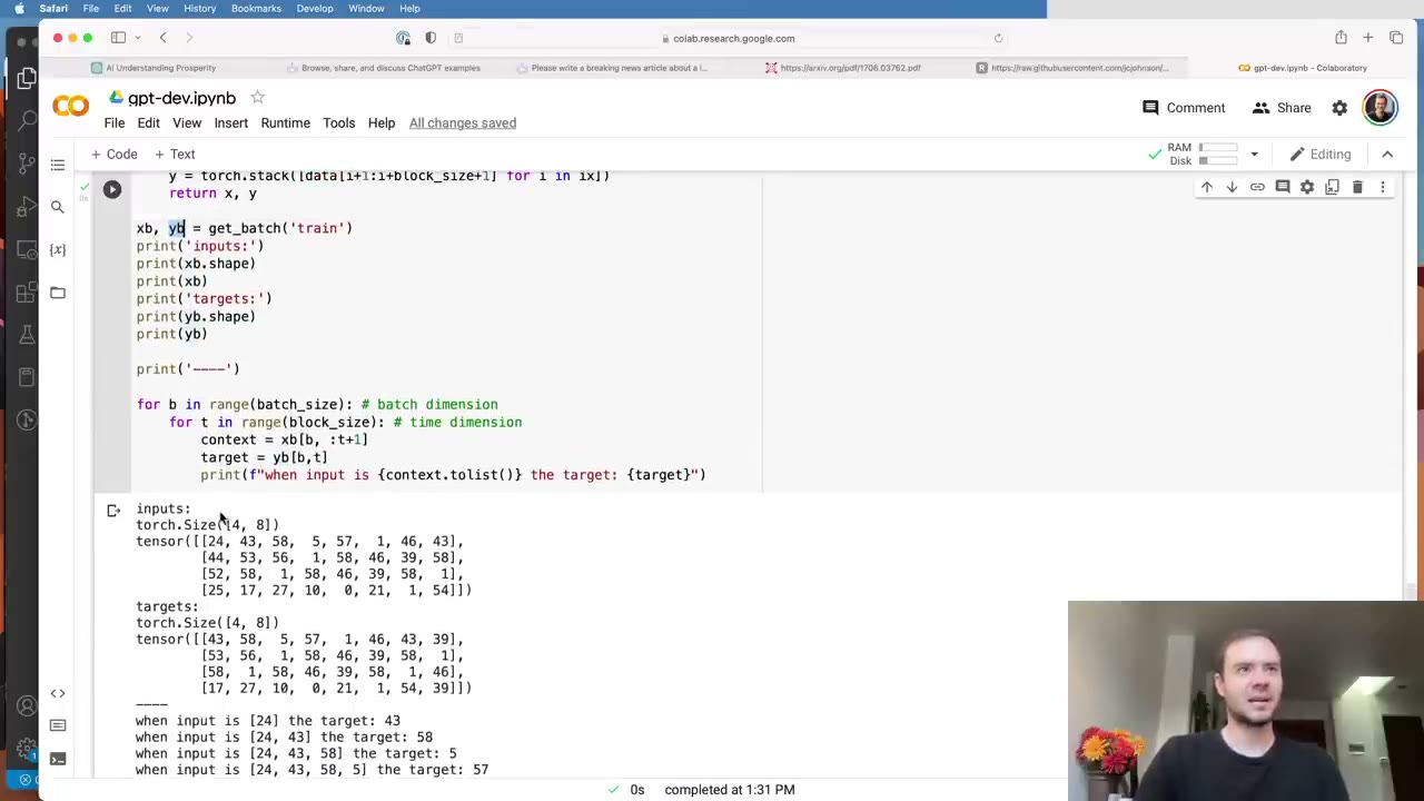20:36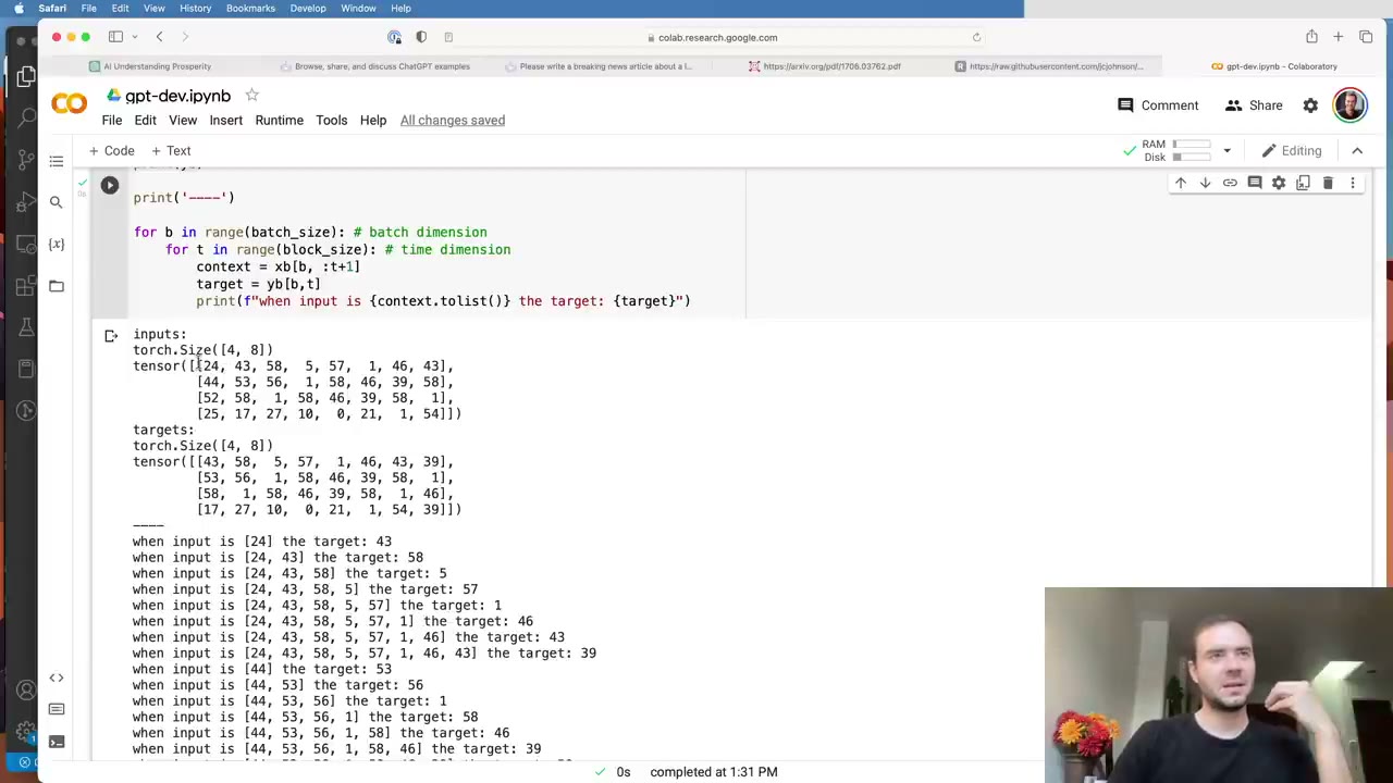21:21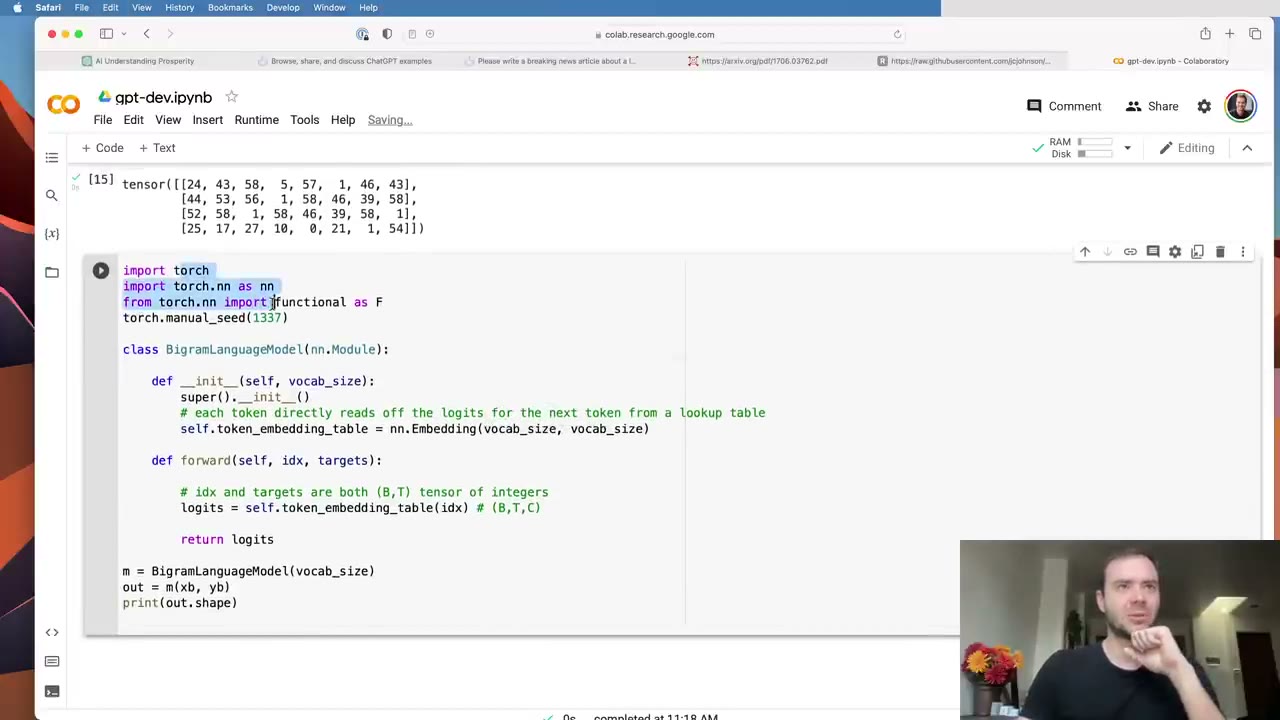22:39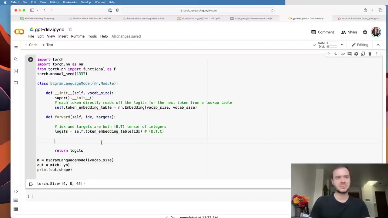25:0926:0526:5228:2730:51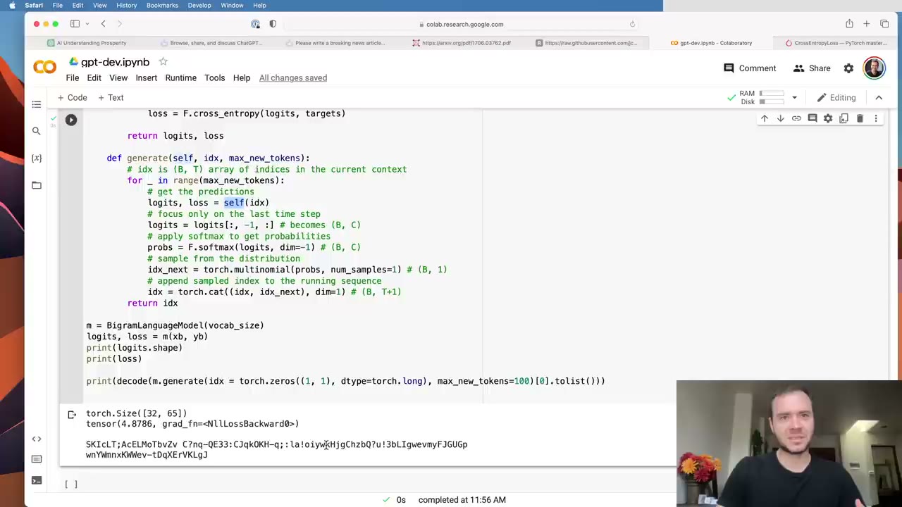34:11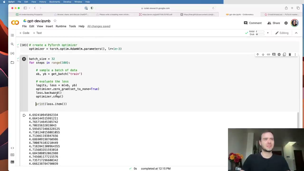36:20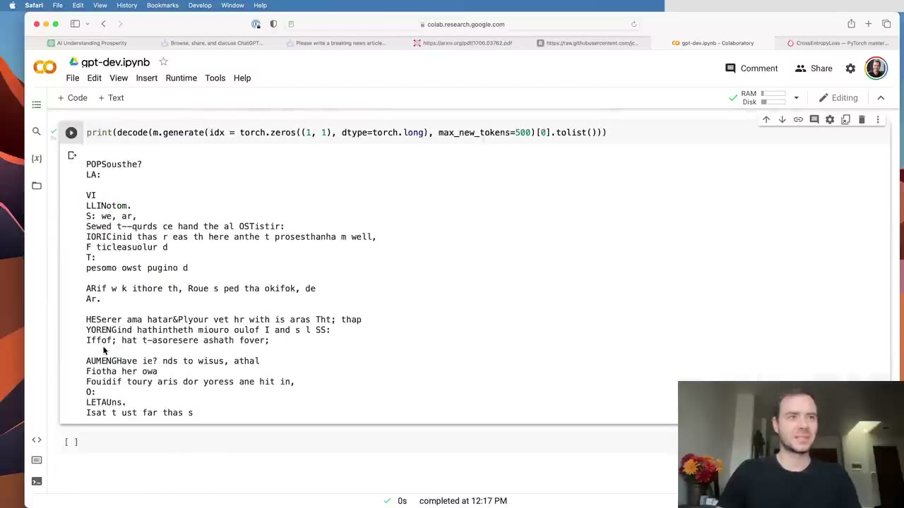37:43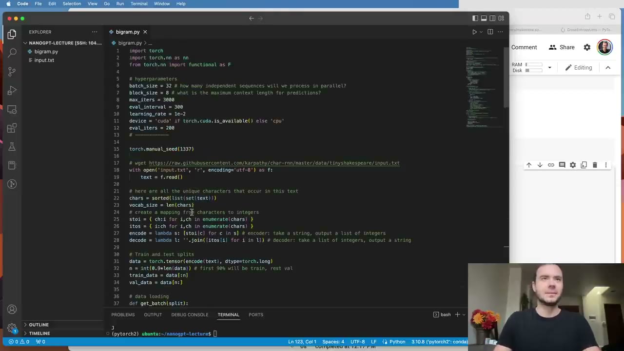38:5640:1341:5442:4646:5747:2551:0152:3254:2755:3657:1059:191:01:201:02:181:07:151:07:491:09:081:11:011:11:501:13:471:17:14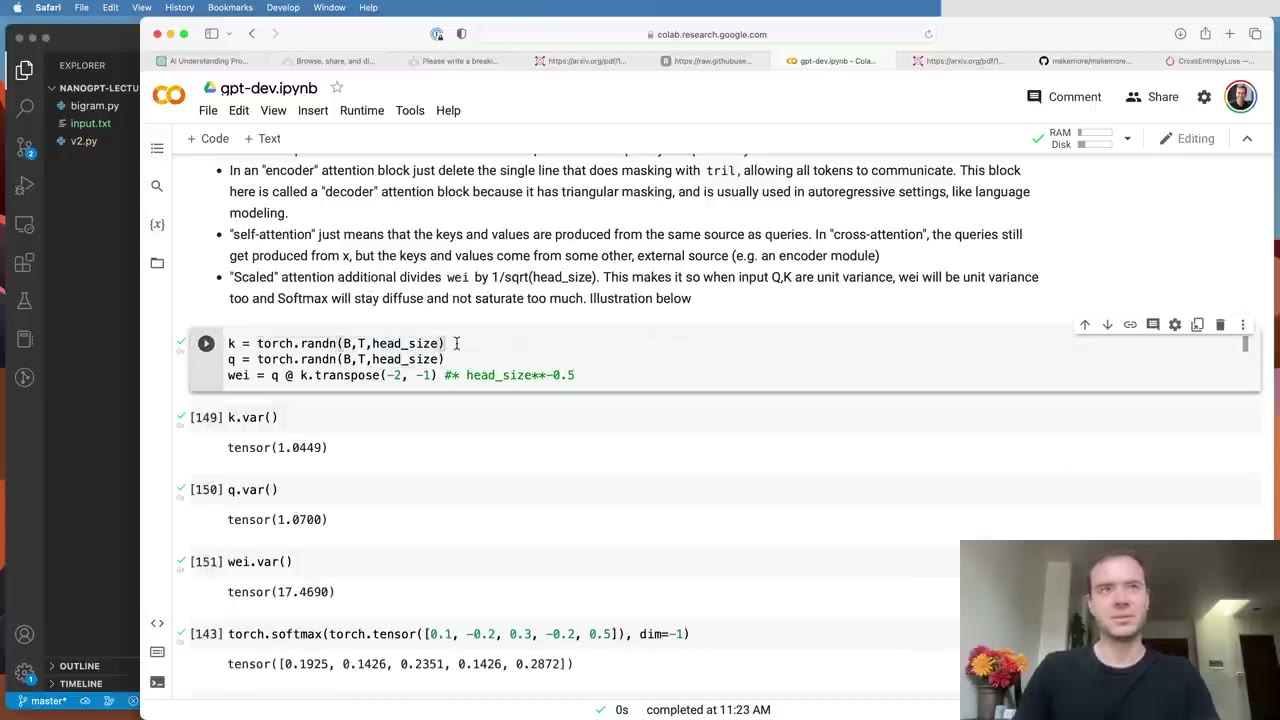1:17:31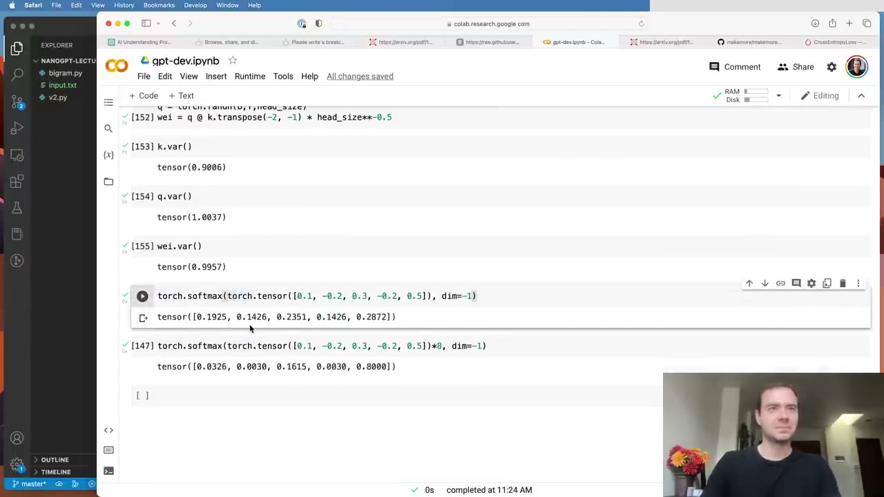1:18:27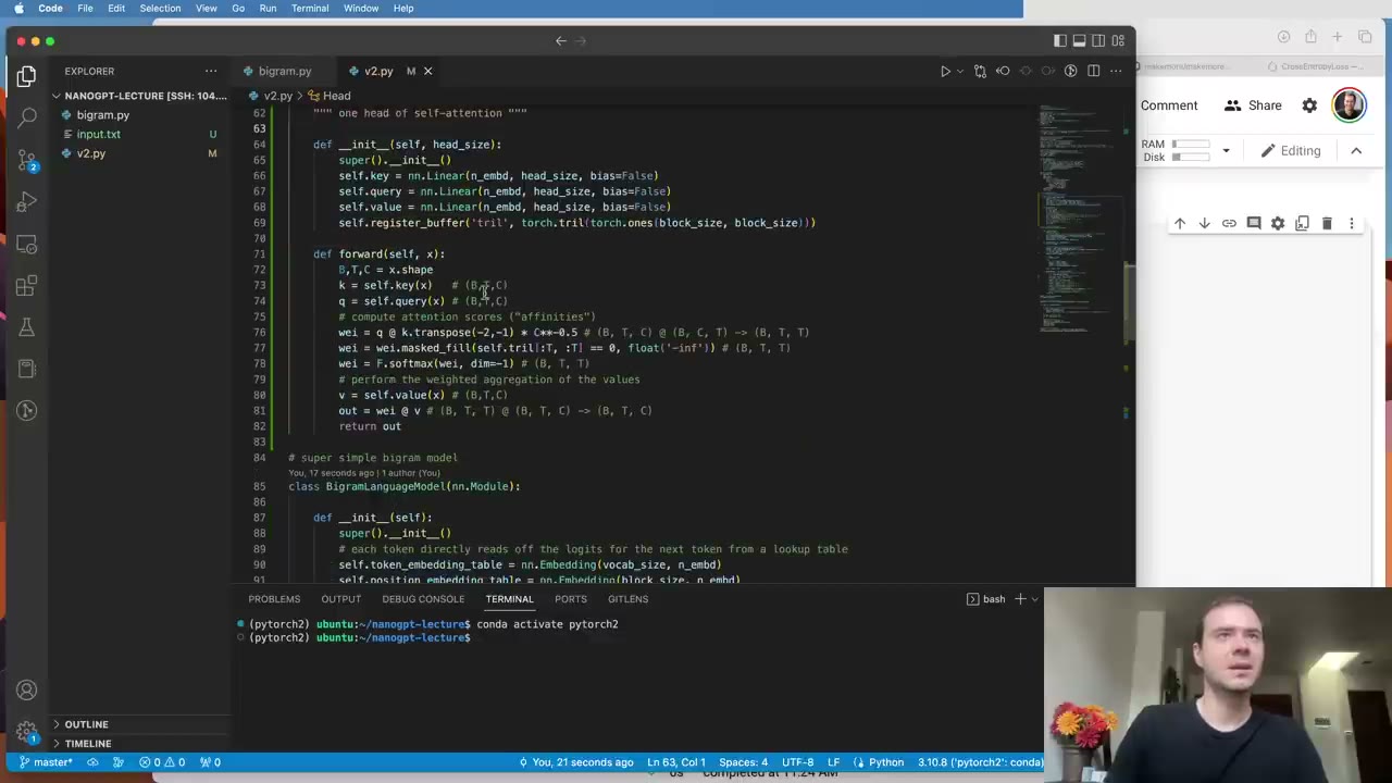1:19:54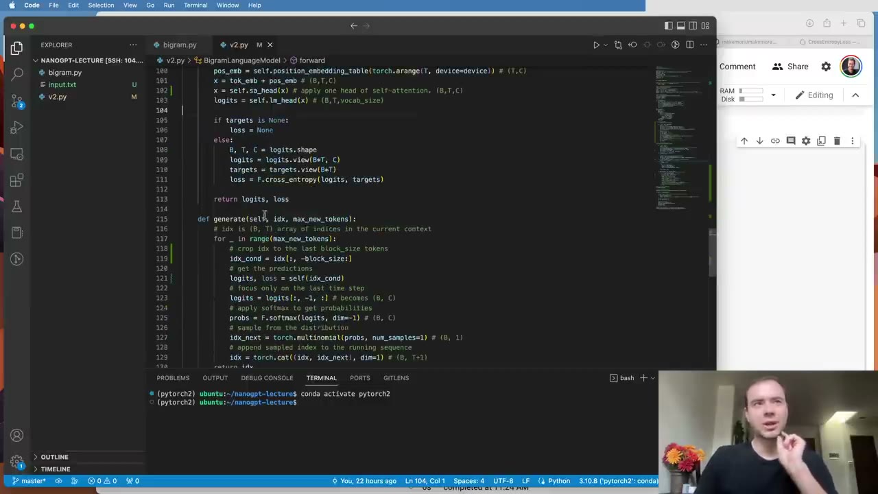1:20:52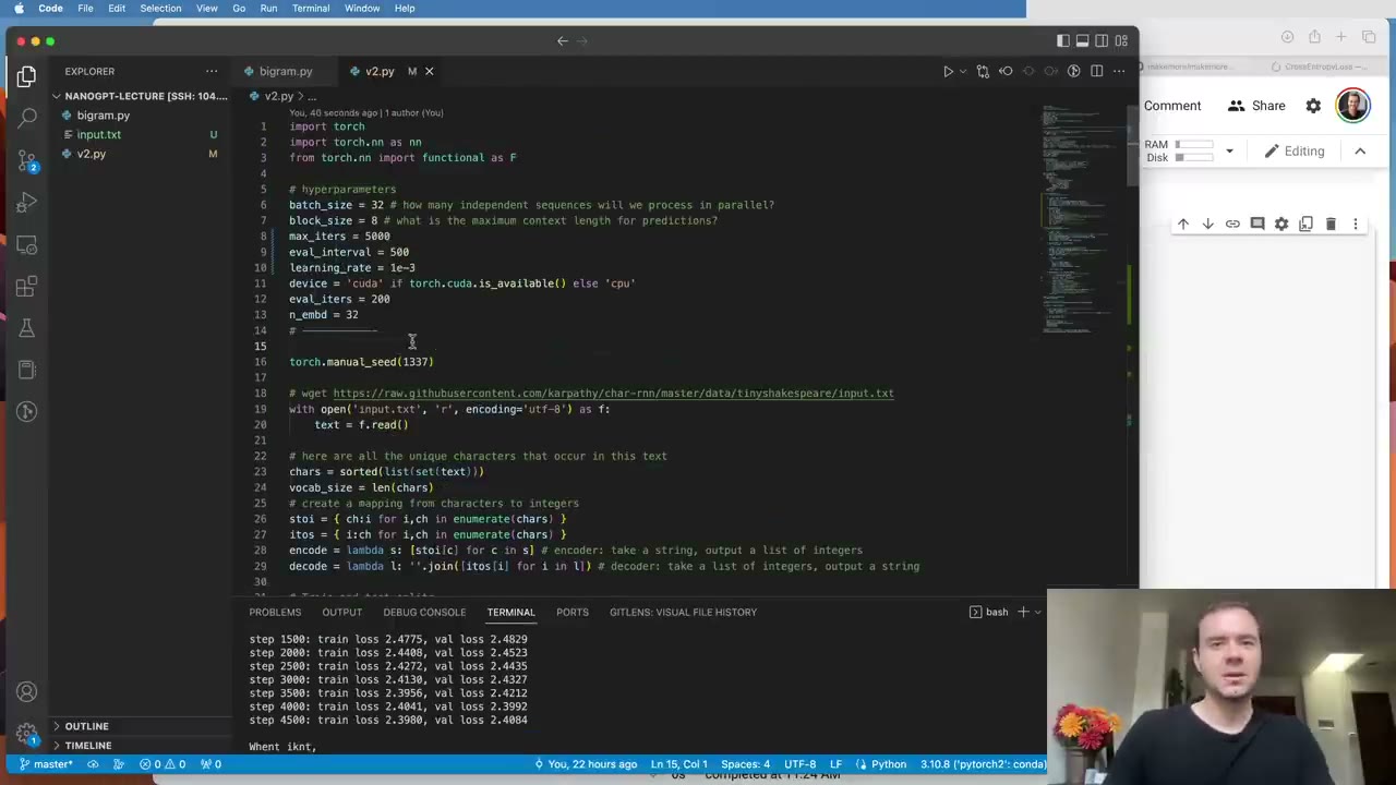1:21:28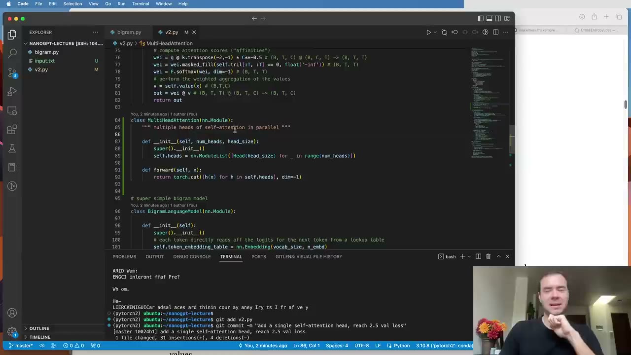1:22:28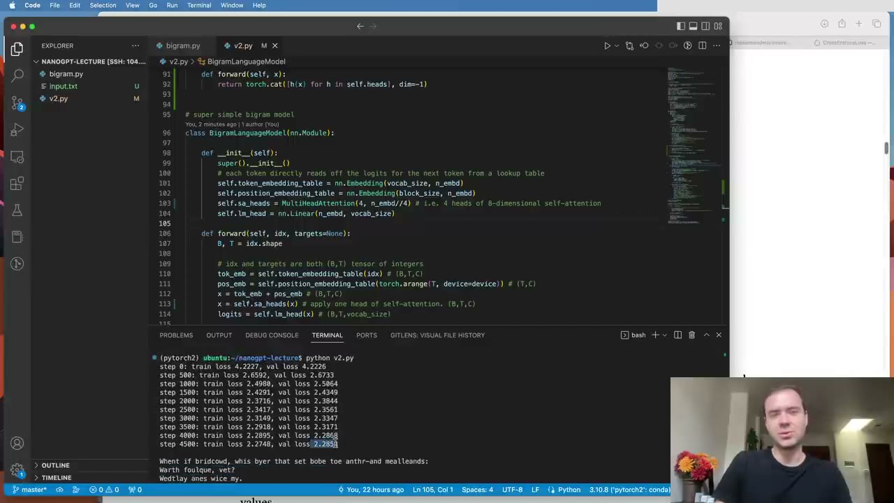1:23:55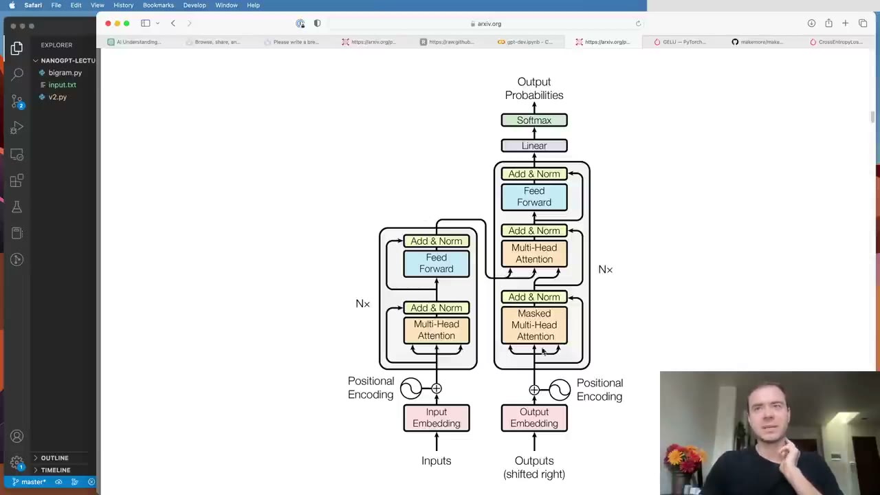1:24:301:25:421:26:581:28:011:28:53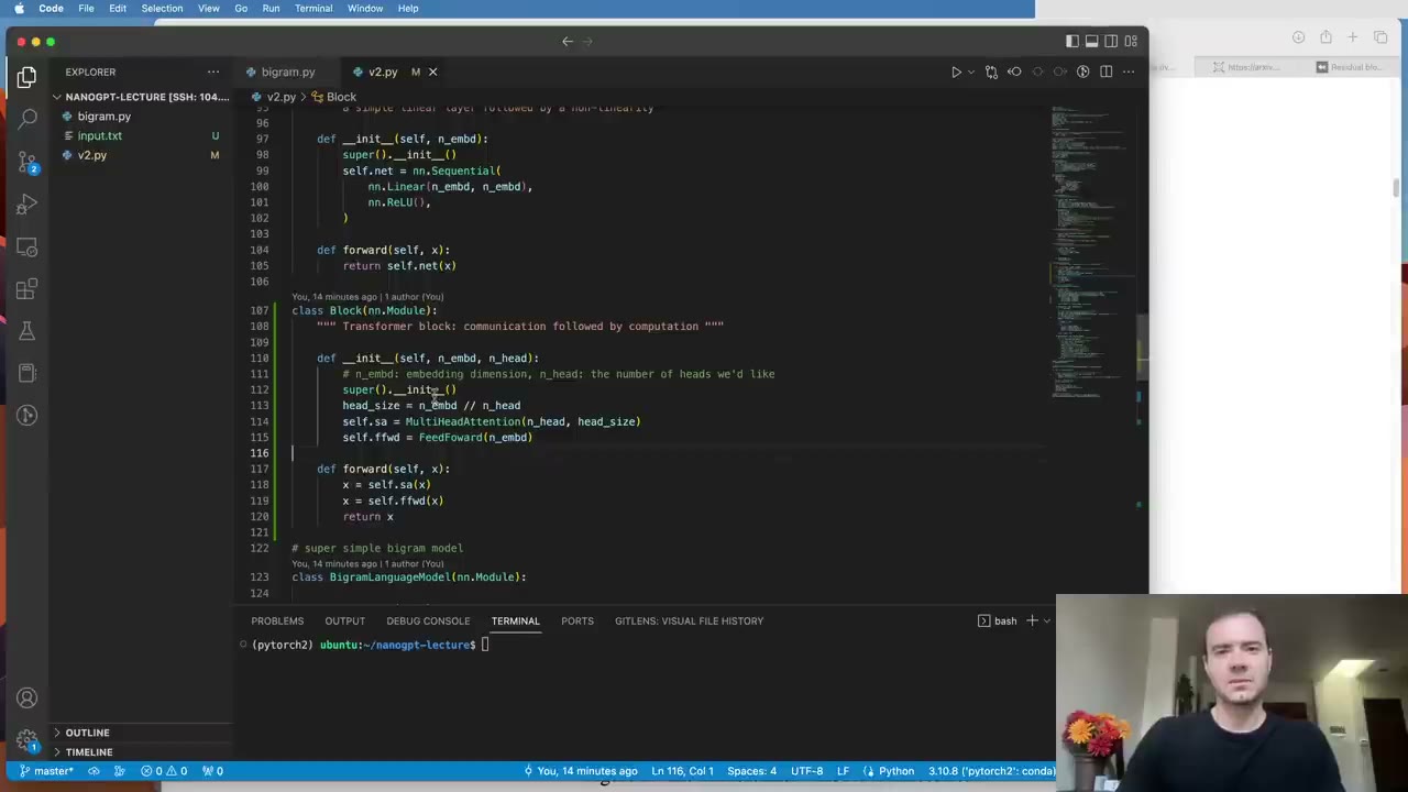1:30:30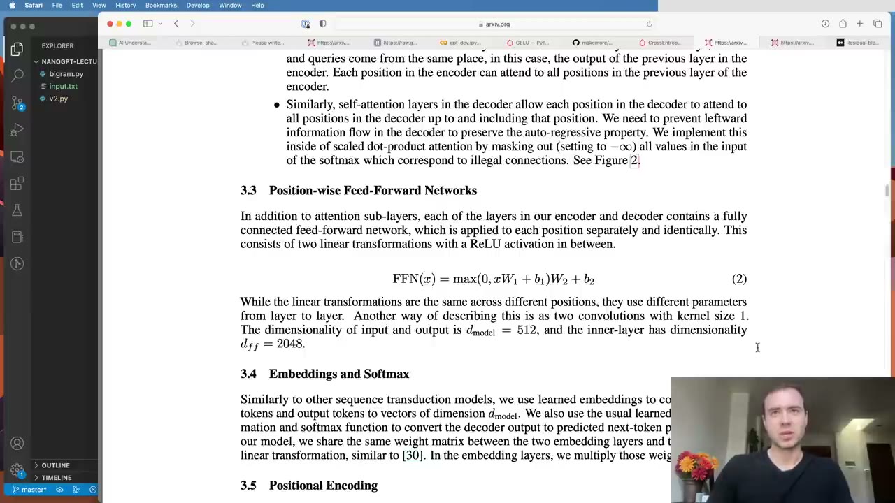1:31:45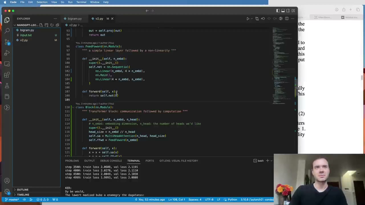1:32:04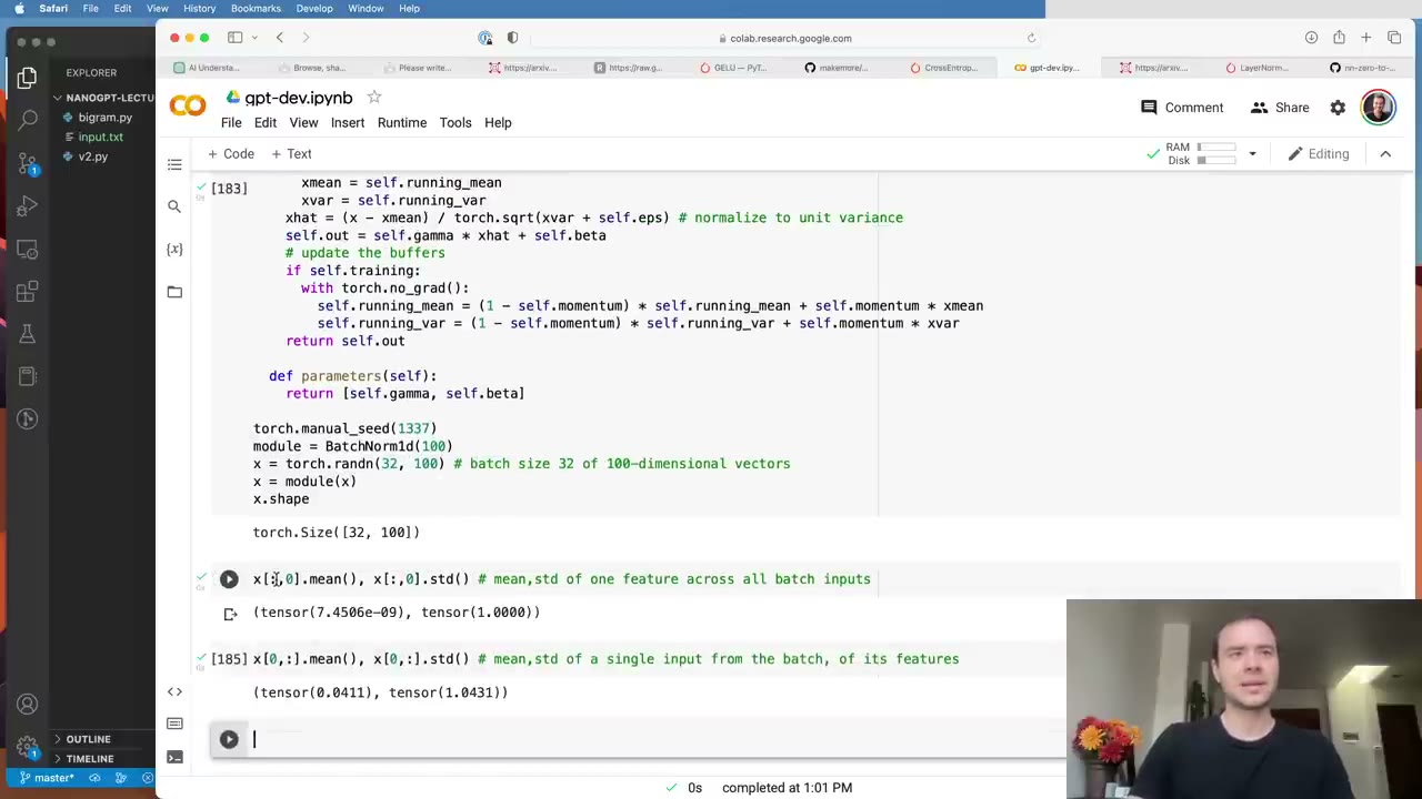1:33:54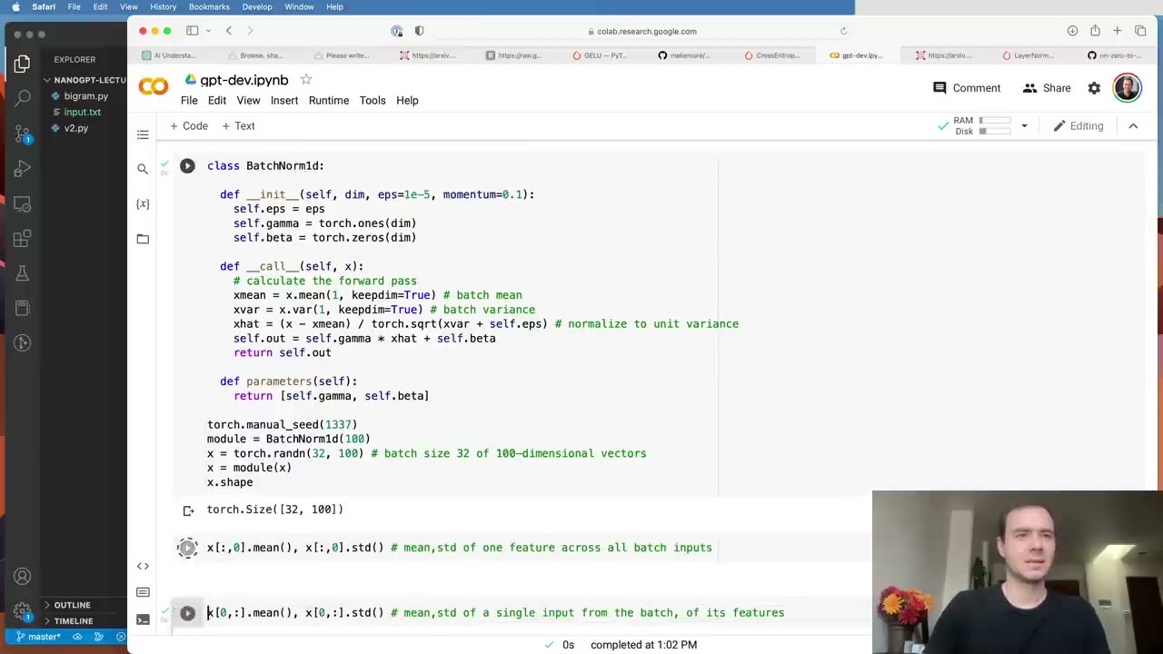1:35:11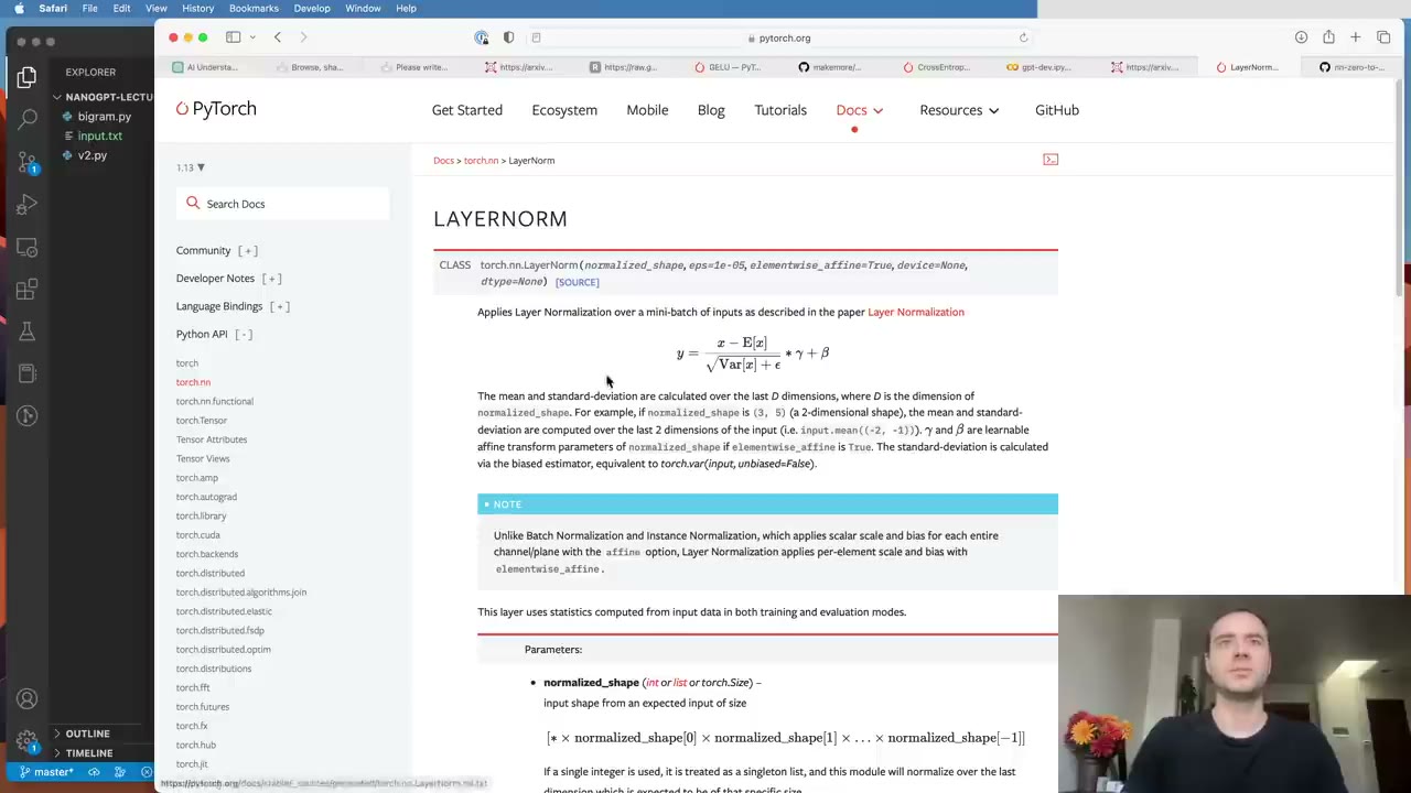1:35:17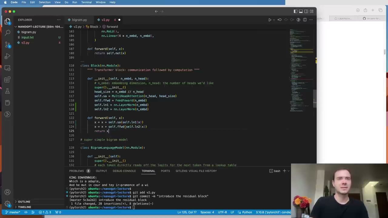1:36:15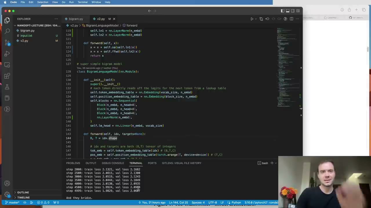1:37:14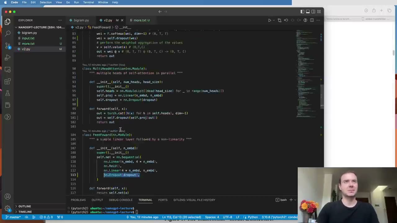1:38:24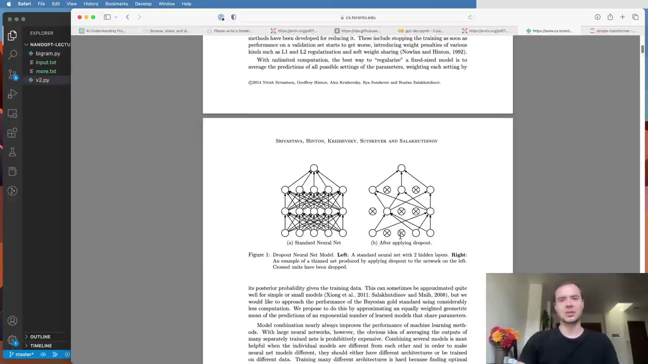1:38:54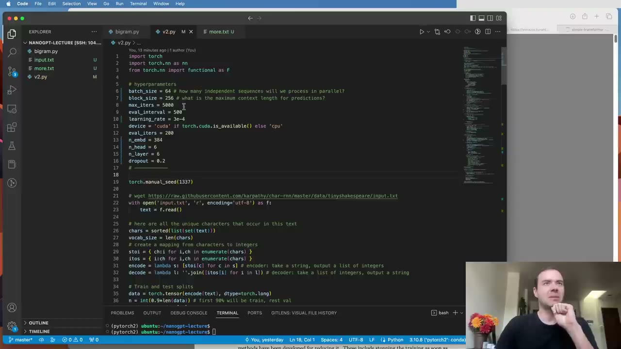1:39:35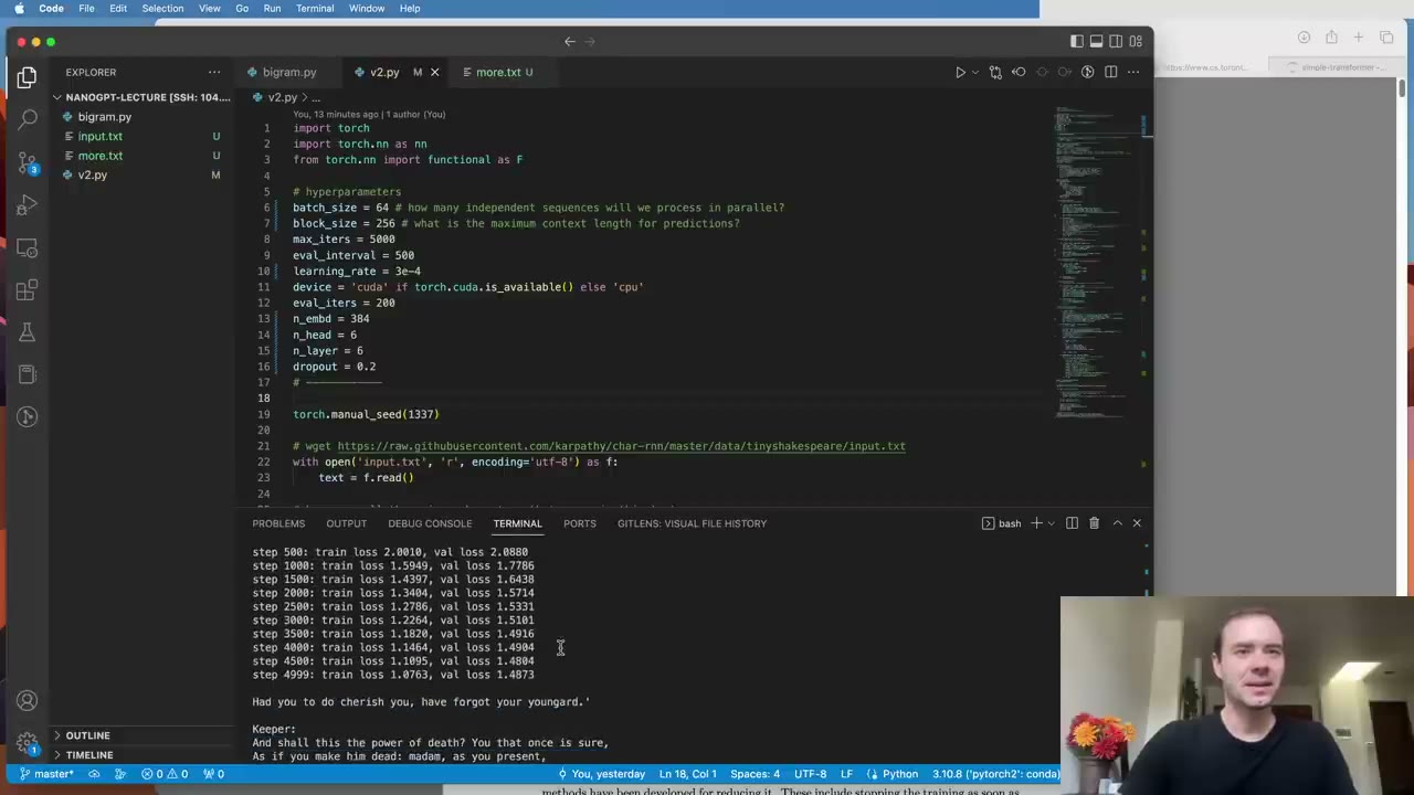1:40:331:41:431:43:201:46:241:47:18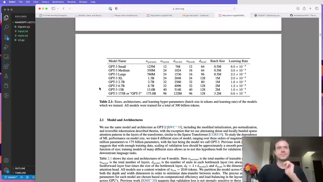1:50:21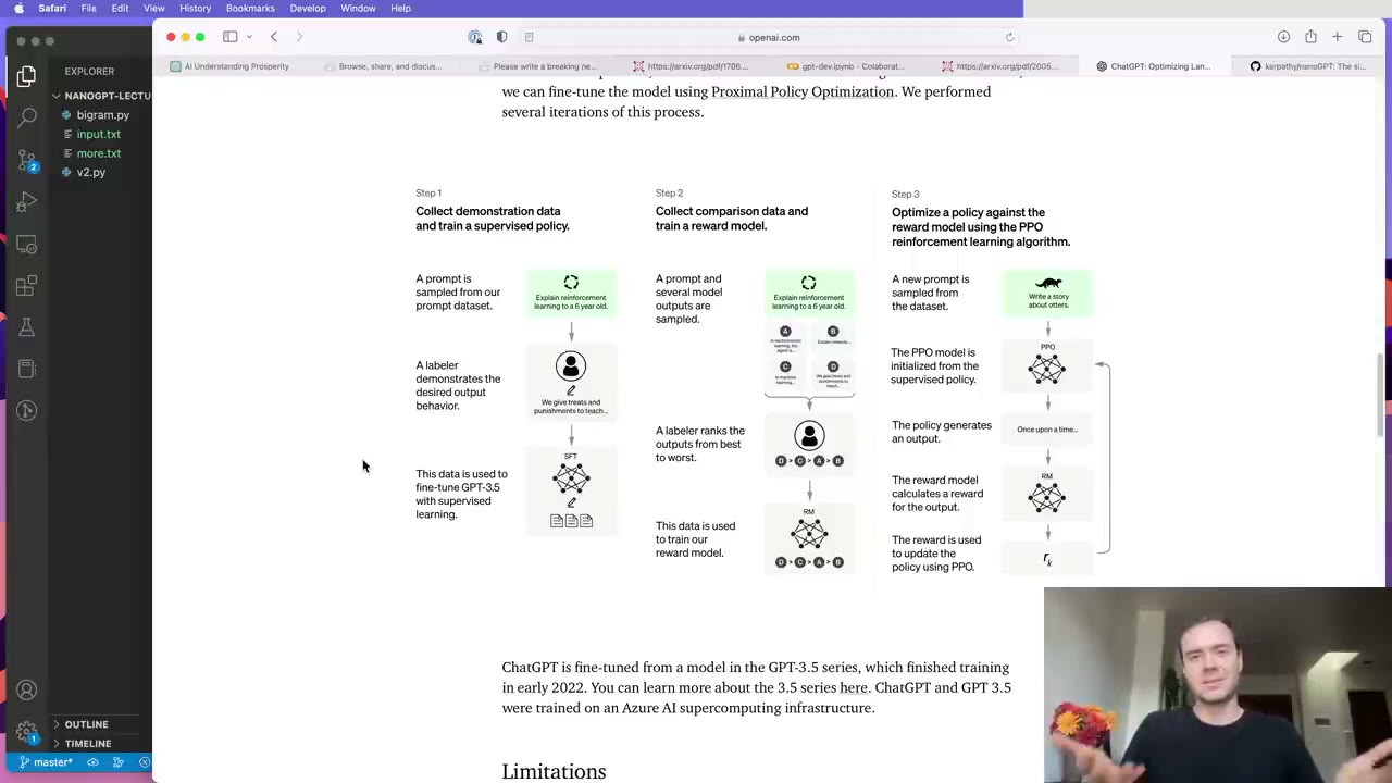1:52:55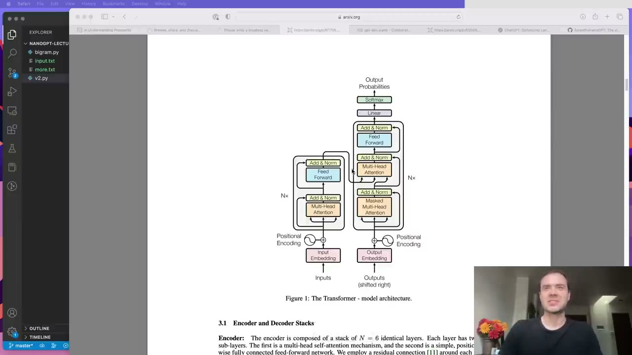1:54:35

Lecture 7 of Andrej Karpathy’s Neural Networks: Zero to Hero is the one most people come for: building a GPT from an empty notebook. After five videos on makemore, the character-level name generator that ended with a WaveNet-style model in Lecture 6, Karpathy switches data sets and architectures. The data is Tiny Shakespeare, about a million characters of plays. The model is a decoder-only Transformer, the architecture from Attention Is All You Need (2017) that sits under ChatGPT. The video moves in a straight line: tokenize the text, train a bigram baseline, learn a matrix trick for averaging over the past, turn that trick into self-attention, then add multiple heads, feed-forward layers, residual connections, LayerNorm and dropout until a scaled-up model writes passable fake Shakespeare. It closes with a tour of nanoGPT and a sketch of how ChatGPT adds fine-tuning on top of pretraining. The tokenizer that real GPTs use, which this lecture deliberately avoids, is the subject of Lecture 8. For the full course map, see the series index.

Key takeaways

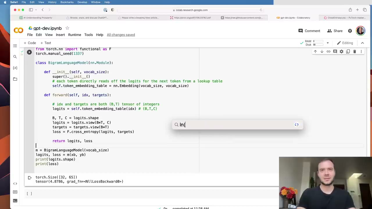
1. One chunk of text is many training examples (15:34). A slice of block_size + 1 characters gives block_size predictions, one for each context length from 1 up to the full block, which also teaches the model to work with short prompts.
2. Check the starting loss against the uniform guess (28:10). With 65 characters, a model that knows nothing should score about −ln(1/65) ≈ 4.17. The untrained bigram scores 4.87, so its first guesses are slightly too confident.
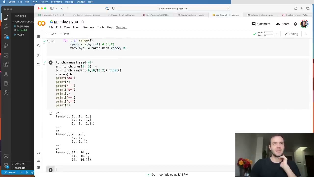
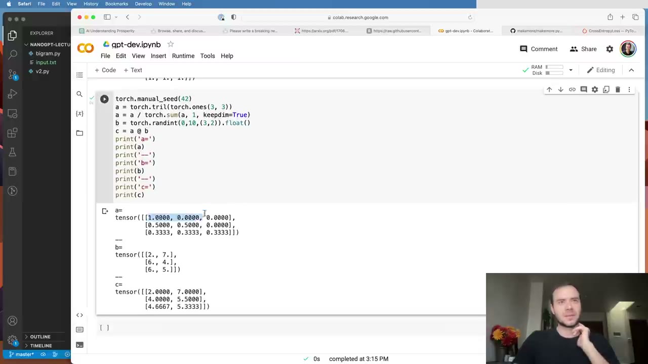
3. Averaging over the past is a matrix multiply (47:10). Multiply by a lower-triangular matrix whose rows sum to 1 and each position gets a weighted average of itself and everything before it, with no loops.
4. Self-attention makes those weights depend on the data (1:03:58). Each token emits a query (what it is looking for) and a key (what it contains); their dot products decide how much of each earlier token’s value flows in.
5. Attention is communication between nodes, with no built-in sense of position (1:11:20). That is why positions must be added as embeddings, and why removing the mask turns a decoder block into an encoder block.
6. Scale the scores by 1/√head_size (1:16:59). Without it, softmax turns nearly one-hot at initialization and each token listens to just one other.
7. Residual connections and LayerNorm make depth trainable (1:28:23). Stacking blocks without them made results worse; with them the validation loss kept falling.
8. Scaling up the same code takes validation loss from about 2.07 to 1.48 (1:40:21). The architecture barely changes; context, width, depth and dropout do the work.

Chapter notes

0:02 – 7:46 ChatGPT, the Transformer and the plan

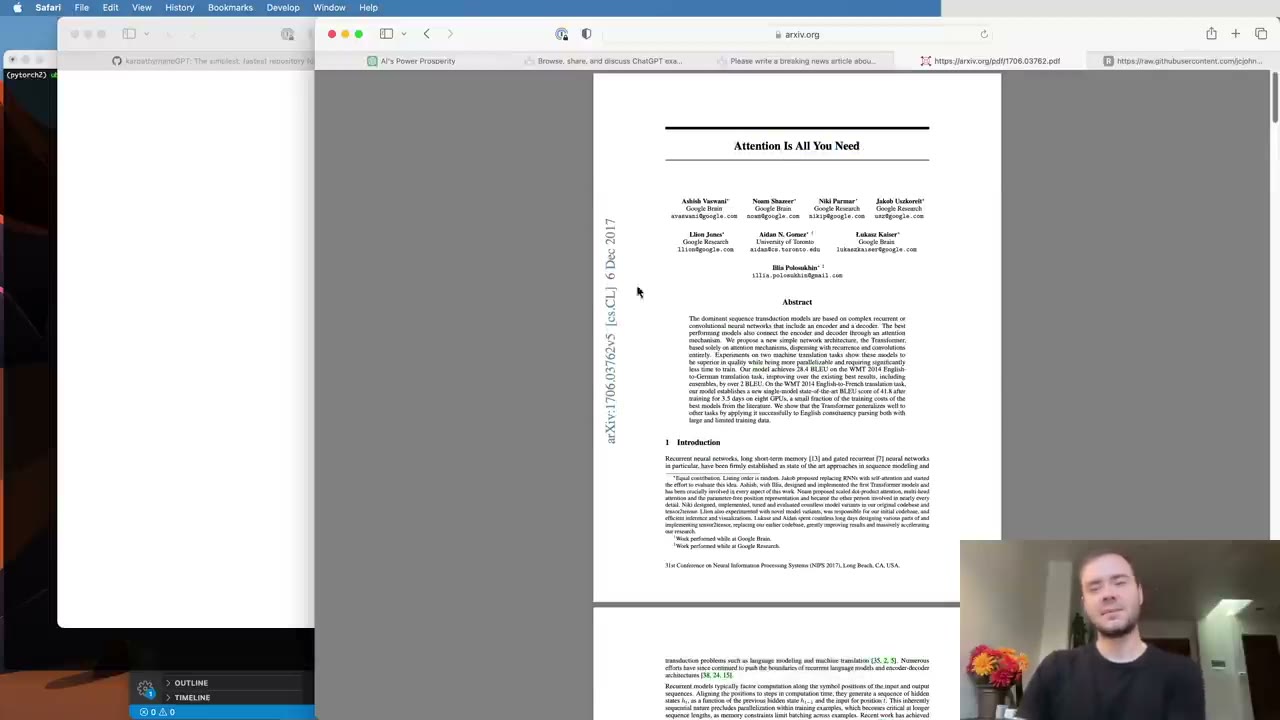
Karpathy opens with ChatGPT writing a haiku twice and getting two different answers, a quick way to show that a language model is a probabilistic sequence completer. The network doing the work comes from the 2017 paper Attention Is All You Need (2:07). He notes that it reads like an ordinary machine-translation paper whose authors probably didn’t foresee that the architecture would spread across most of AI within five years.

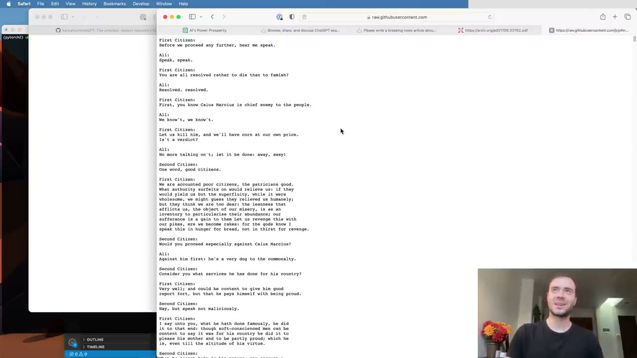
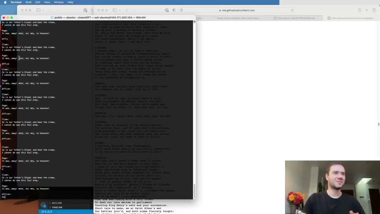
Reproducing ChatGPT is out of reach, so the goal is narrower: train a character-level Transformer language model on Tiny Shakespeare, roughly 1 MB of plays in one file (3:40). He previews the end result, an endless stream of fake Shakespeare produced one character at a time, and points out that ChatGPT works the same way except on subword tokens.

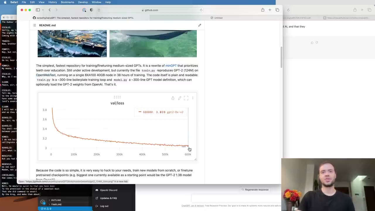
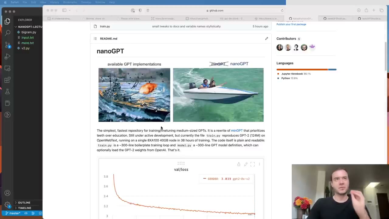
He also introduces nanoGPT (5:43), his two-file repository (one file for the model, one for training) that reproduces the smallest GPT-2, the 124M-parameter model, on OpenWebText. This lecture rebuilds its core from an empty file. Prerequisites are Python, basic calculus and statistics, and ideally the makemore videos (7:16).

Our note: Karpathy dates GPT-2 to 2017, adding “if I recall correctly”. OpenAI released it in 2019; 2017 is the year of the Transformer paper.

7:46 – 13:29 Reading the data and building a tokenizer

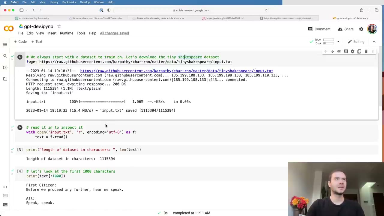
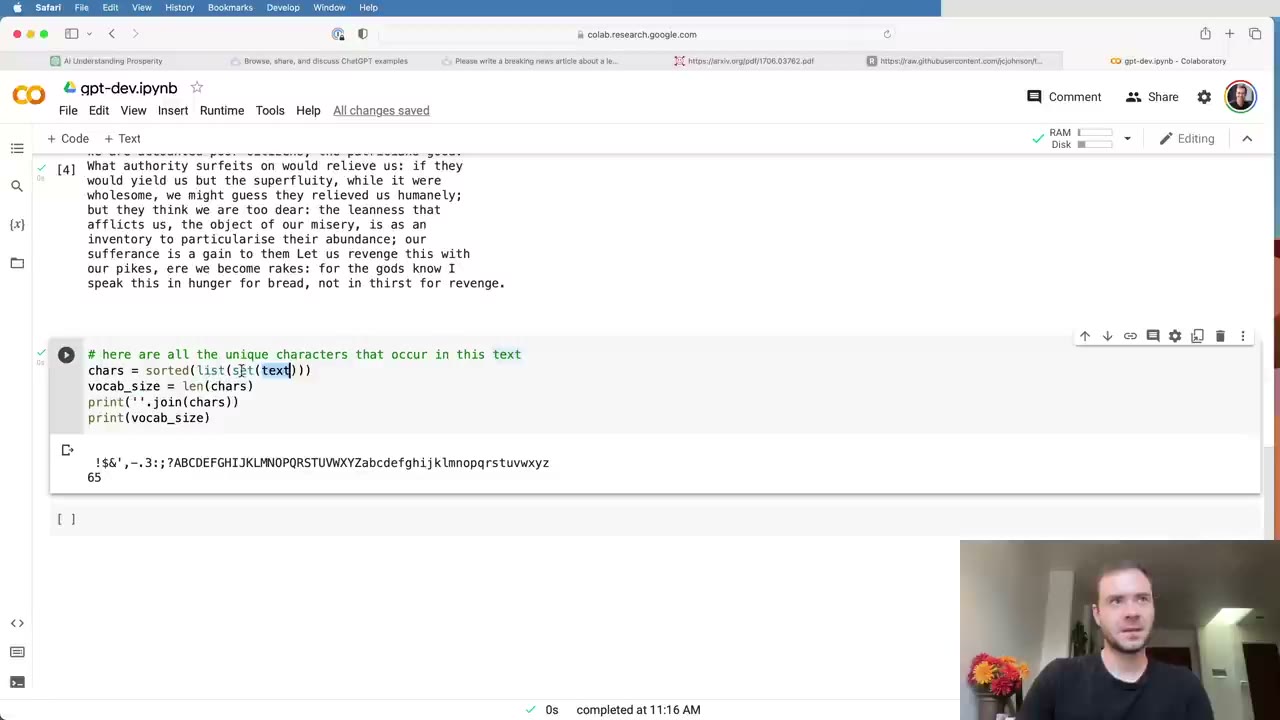
In a Google Colab notebook he downloads the file, reads about a million characters, and collects the sorted set of distinct characters: 65 in all, covering space, punctuation, and upper- and lowercase letters (8:49). That set is the vocabulary.

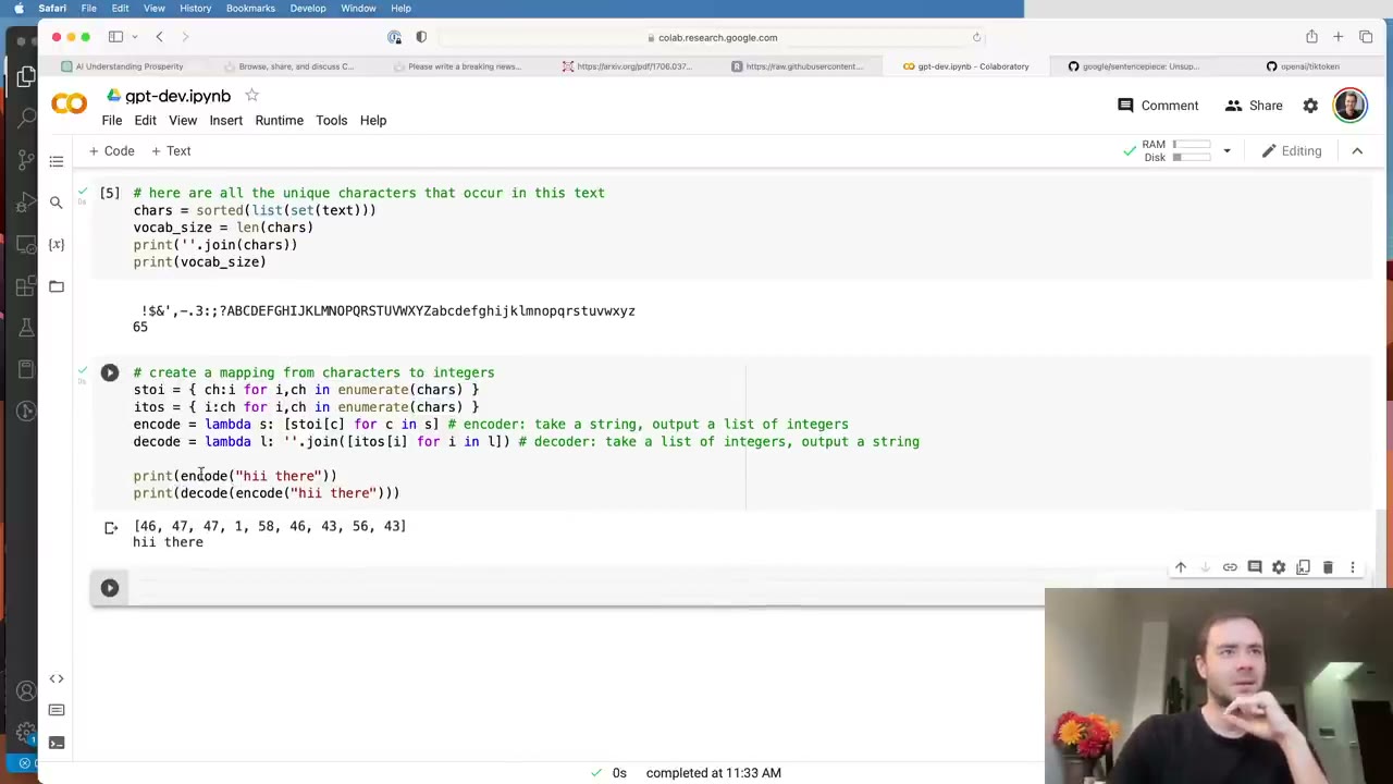
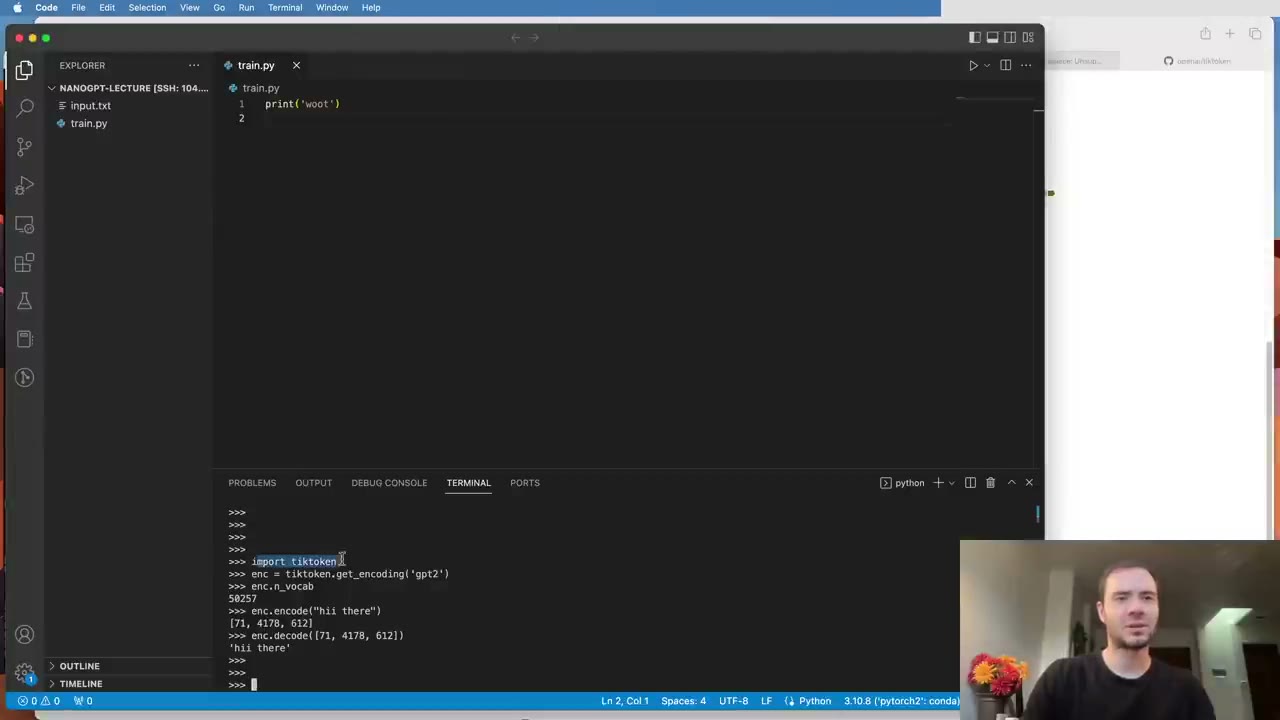
Tokenizing means turning text into a sequence of integers. Here it is the simplest possible scheme: two lookup tables, character to integer and back, with encode and decode built on them (9:53). He contrasts it with what production systems use. Google’s SentencePiece and OpenAI’s tiktoken both work on subword units; with the GPT-2 encoding, the on-screen string “hii there” becomes three integers drawn from a vocabulary of about 50,000 instead of nine from a vocabulary of 65 (11:24). The trade-off is vocabulary size against sequence length, and he keeps characters because they make everything else easy.

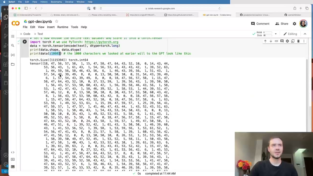
The whole text is then encoded and wrapped in a torch.tensor, so from here on Shakespeare is just one long row of integers.

13:29 – 21:51 Train/val split, block size and batches

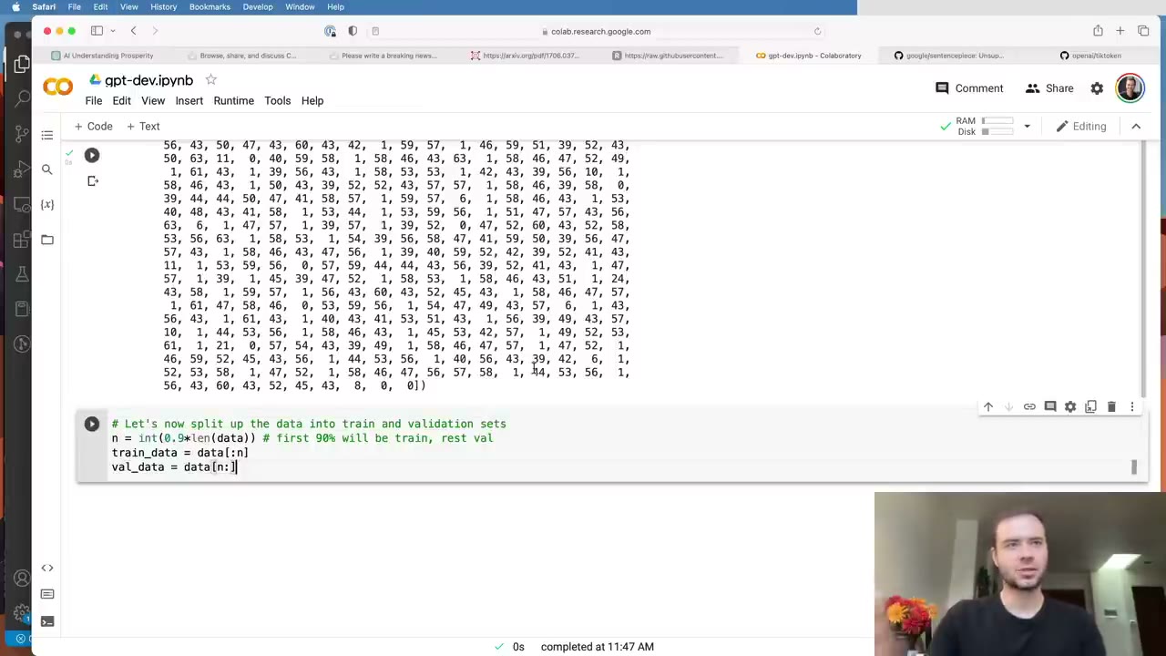
The first 90% becomes training data and the last 10% validation data (13:29), so overfitting can be measured: the goal is text that looks like Shakespeare, not memorized Shakespeare.

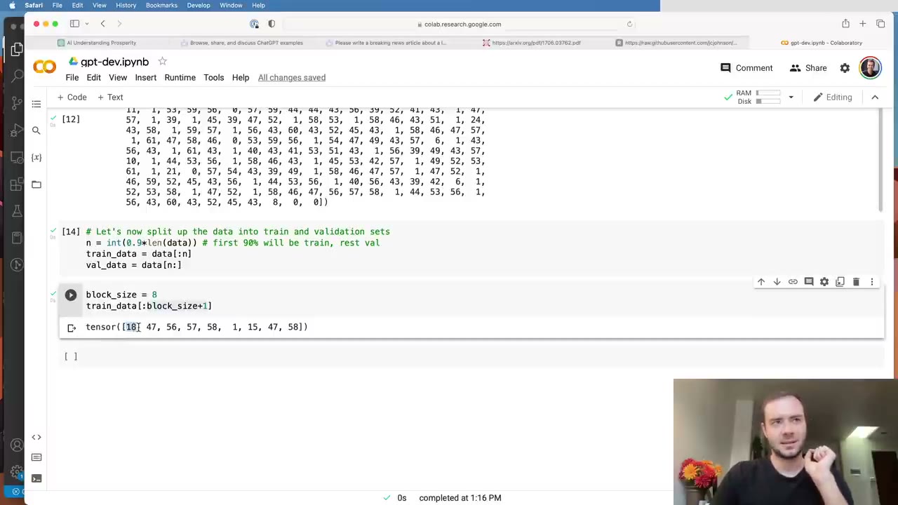
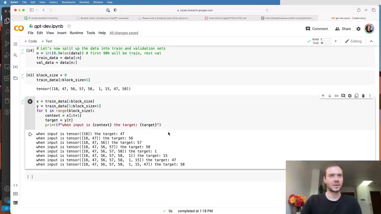
The Transformer never sees the whole text at once. It trains on random chunks no longer than block_size, which other code bases call the context length (15:01). With block_size = 8, he grabs nine characters and spells out the eight examples inside them: given the first character predict the second, given the first two predict the third, and so on (16:37). Training on every context length isn’t only about efficiency. It means that at generation time the model can start from a single character, and it explains why generation must later crop its input to block_size.

The second dimension is the batch (18:11). Several chunks are stacked into one tensor purely to keep the GPU busy; they never interact. get_batch picks random offsets, stacks the inputs into a 4×8 tensor x, and stacks the same windows shifted by one into the targets y (18:42). One such batch holds 32 independent examples.

21:51 – 28:40 A bigram baseline and its loss

The simplest language model, covered in depth in makemore, is the bigram: predict the next character from the current one alone. Karpathy writes it as an nn.Module whose only part is an nn.Embedding of size vocab × vocab (22:53). Each input integer plucks out one row, and that row is read directly as the logits, the scores for the next character. The output is a batch × time × channel (B, T, C) tensor, a naming convention used for the rest of the video.

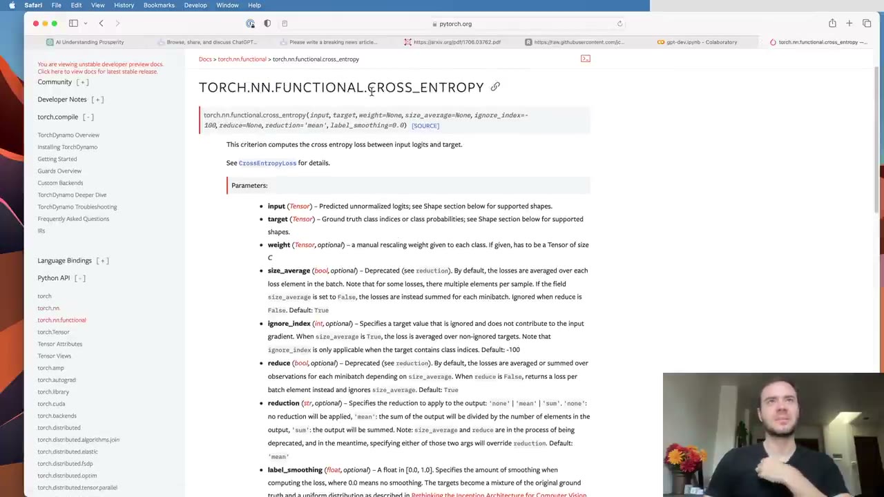
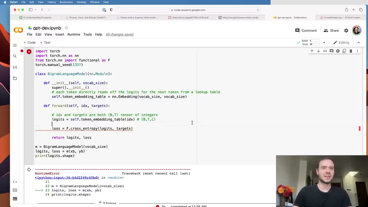
For the loss he uses F.cross_entropy, PyTorch’s negative log likelihood on logits (25:00). It fails at first because PyTorch wants the channel dimension second for multi-dimensional input. Rather than permute, he flattens: logits become (B·T, C) and targets (B·T) (26:35). The first loss is 4.87 against an expected 4.17 for uniform guessing (28:10), so the random initialization is a bit off but usable.

28:40 – 37:50 Generating text and training with AdamW

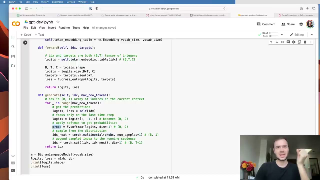
generate takes a (B, T) tensor of indices and appends max_new_tokens new ones (29:11). Each step runs the model, keeps only the logits at the last time position, applies softmax, samples one index with torch.multinomial and concatenates it on. Targets become optional in forward so the model can run without them. Starting from a single 0 (the newline character), the untrained model produces garbage (33:32).

He admits the function looks wasteful for a bigram, feeding the whole history only to use the last character (34:05). It is written that way so it won’t need to change once the model actually uses its history.

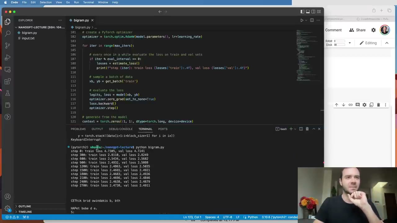
Training swaps the plain gradient descent of makemore for AdamW (34:35). He gives 3e-4 as a typical learning rate and says small networks tolerate much higher ones. The loop is the familiar four steps: sample a batch, compute the loss, zero the gradients, backpropagate and step. After 10,000 steps the loss settles near 2.5 and the samples start to look vaguely like text (36:48). The limitation is obvious: tokens don’t talk to each other.

37:50 – 41:59 From notebook to script

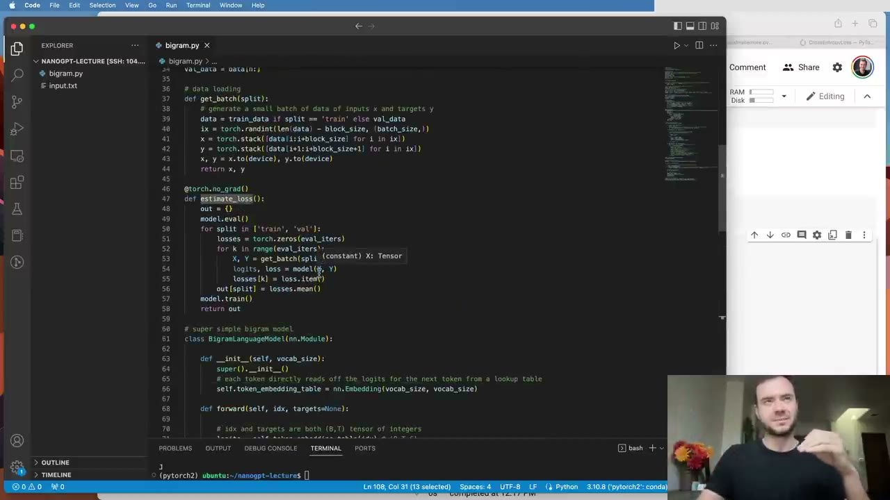
The notebook becomes bigram.py, about 120 lines, with hyperparameters at the top (37:50). Three additions matter later. The code runs on a GPU when available, which means moving the data, the model and the generation context to device. An estimate_loss function averages the loss over many batches for both splits (39:54), because a single batch’s loss is noisy. And that function switches the model to eval mode and back, and runs under @torch.no_grad() so PyTorch doesn’t store intermediate values for a backward pass that never comes (40:26). Neither mode switch changes this model yet, but dropout will need it later.

41:59 – 58:12 The mathematical trick behind self-attention

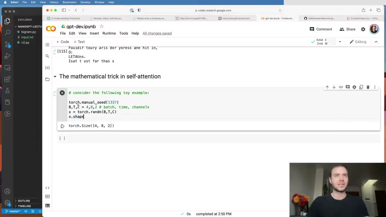
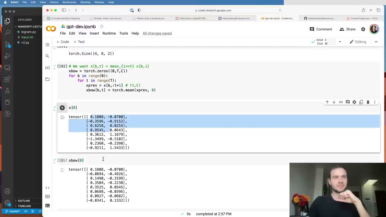
Before writing attention, Karpathy isolates the operation at its core using a toy (B, T, C) = (4, 8, 2) tensor (42:30). The goal is for each token to gather information from earlier positions, and only those, since future tokens are what the model must predict. The crudest version is to average the vectors of all previous tokens and the current one, a “bag of words” (45:05). It throws away order, but it is a start.

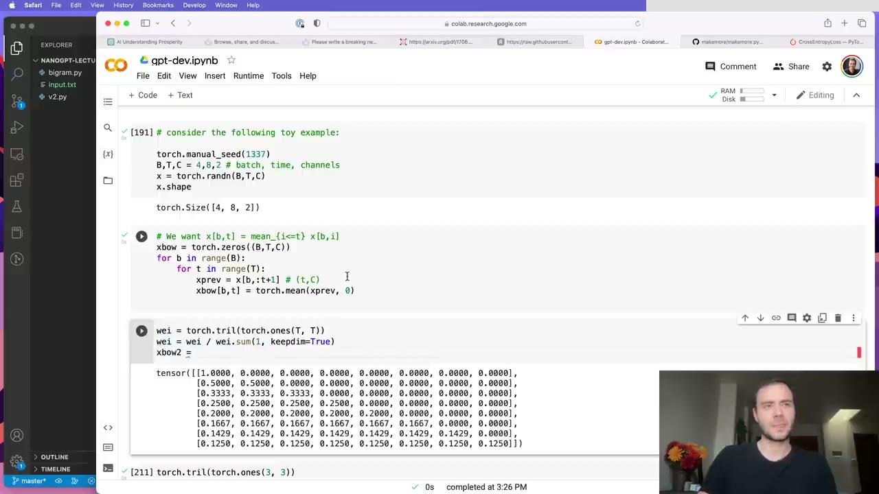
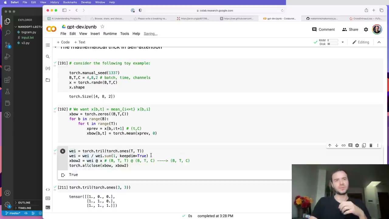
The loop version is slow, so he shows the trick with small matrices (47:10). Multiplying by a matrix of ones sums the columns of the second matrix. Keeping only the lower triangle with torch.tril makes row t sum only the first t rows. Normalizing each row to sum to 1 turns those sums into running averages (50:23). Applied to the toy data, a (T, T) weight matrix wei times the (B, T, C) input broadcasts into a batched matrix multiply and reproduces the loop’s output exactly (51:59).

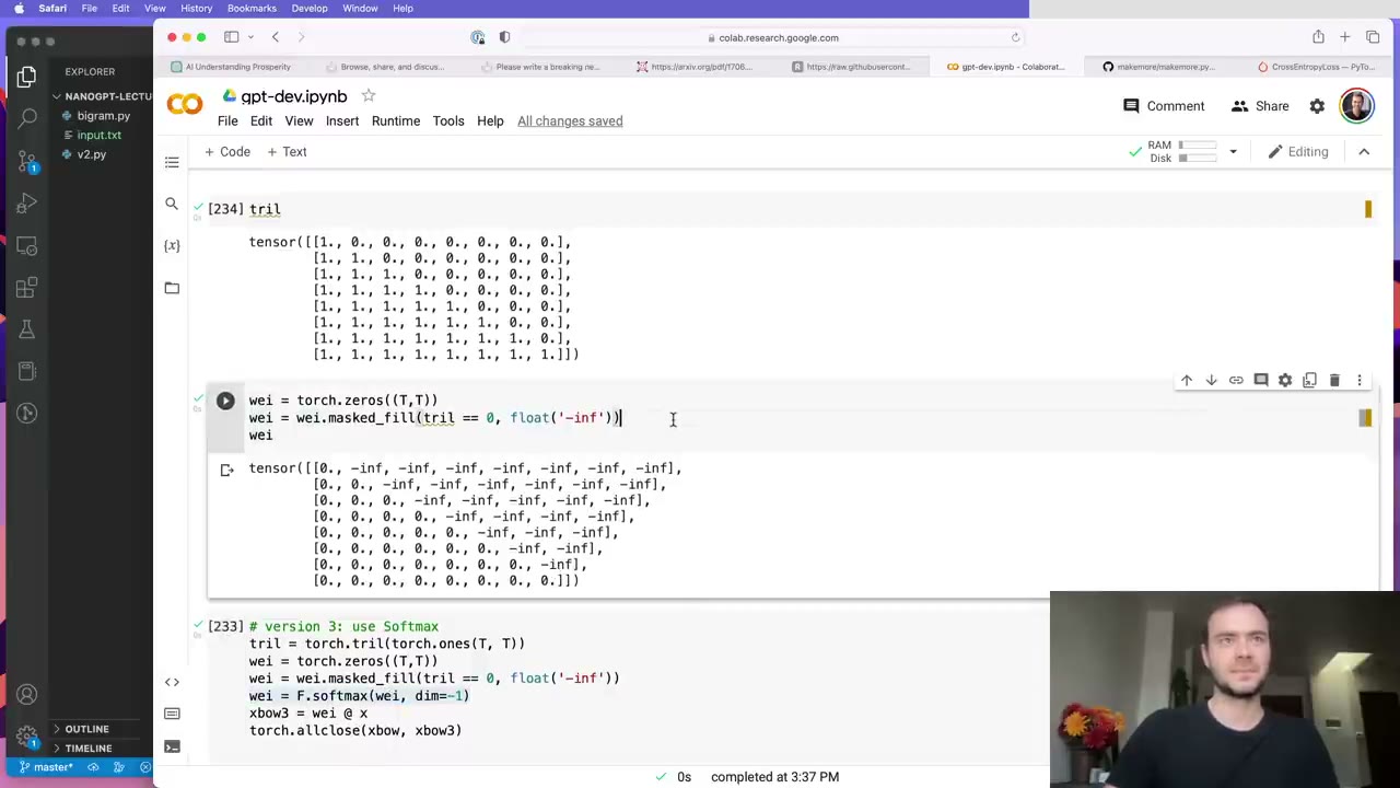
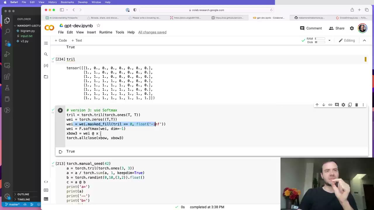
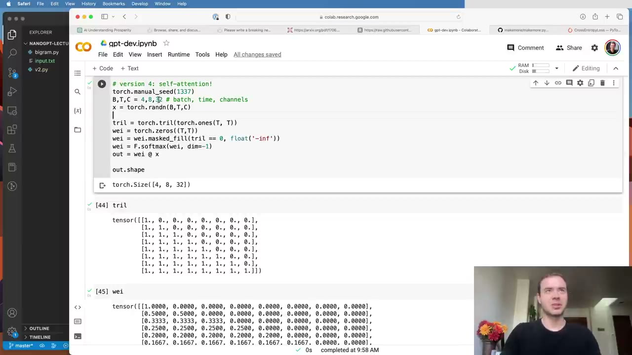
The third version is the one that carries forward (54:33): start wei at zeros, use masked_fill to set the upper triangle to −∞, then apply softmax along each row. The result is the same averaging matrix, but now it reads differently. The zeros are affinities, how interested one token is in another; the −∞ entries forbid talking to the future; softmax turns affinities into weights (56:37). Self-attention will simply compute the affinities from the data instead of fixing them at zero.

58:12 – 1:01:52 Embedding width and position embeddings

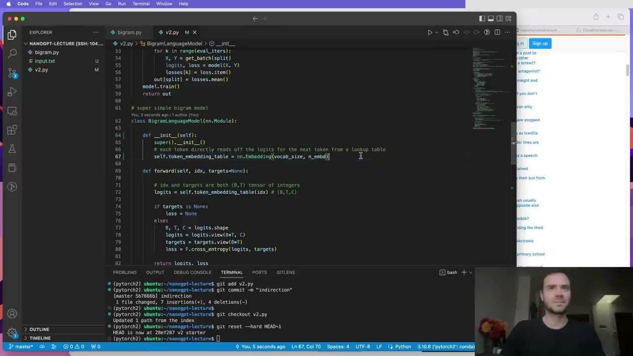
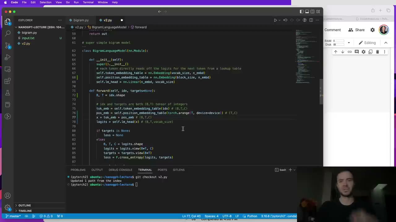
Some groundwork in the script. A new hyperparameter n_embd (32 for now) sets the width of the token embeddings, and a linear layer lm_head maps them to vocabulary logits (58:44). A second table, position_embedding_table of size block_size × n_embd, gives each position from 0 to T−1 its own vector, added to the token embedding through broadcasting (1:00:19). For a bigram this changes nothing, since every position is treated the same, but attention will need it.

1:01:52 – 1:11:20 One head of self-attention

Karpathy flags this as the most important part of the video (1:01:52). Uniform weights treat every past token as equally relevant, but a vowel might want to find consonants, and that preference should depend on content (1:03:27).

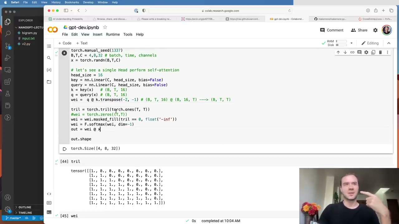
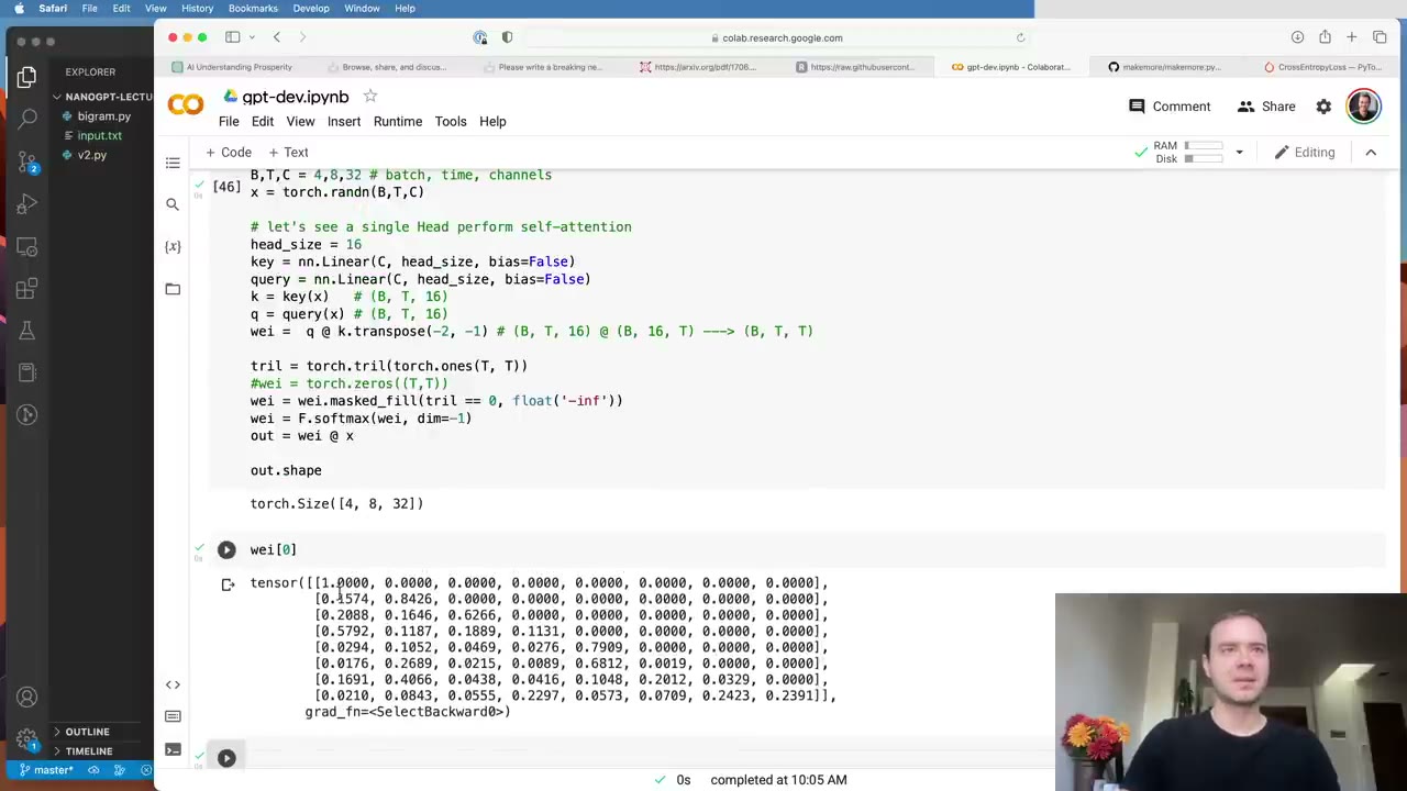
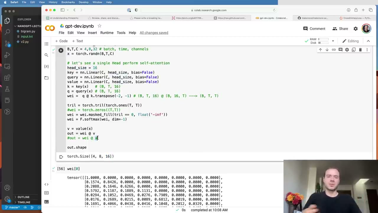
The mechanism (1:03:58): every token emits a query, roughly “what am I looking for”, and a key, roughly “what do I contain”. The affinity between two tokens is the dot product of one’s query with the other’s key. In code, two bias-free linear layers of head_size 16 produce k and q for every position independently, and the communication happens in q @ k.transpose(-2, -1), which gives a (B, T, T) matrix of scores (1:06:07). Unlike the fixed averaging matrix, every batch element now gets its own weights.

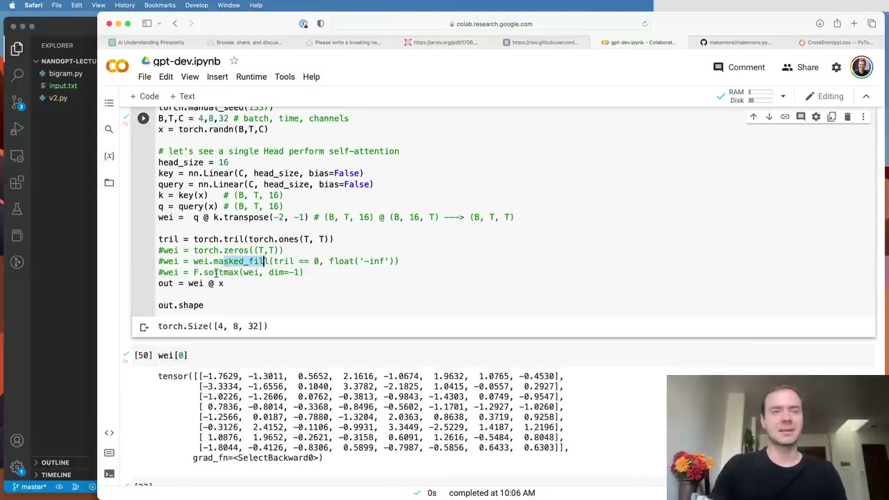
He walks through the eighth token of one example (1:07:41) and then removes the mask and softmax to show the raw scores, which range from about −2 to 2 (1:08:43). Masking blocks the future; softmax turns the rest into a distribution.

The last piece is the value (1:09:45). Tokens don’t share their raw x; a third linear layer produces v, and the output is wei @ v. Karpathy’s framing: x is the token’s private information, and v is what it chooses to tell others who find it interesting.

1:11:20 – 1:16:59 Five notes on attention

A short conceptual pause, worth re-watching.

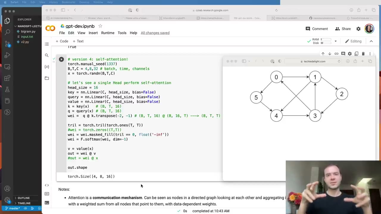
• Attention is a communication mechanism (1:11:20). Picture nodes in a directed graph, each aggregating a weighted sum from the nodes that point to it. In language modeling, node t is pointed to by nodes 1 to t, but any graph is possible.

• There is no notion of space (1:12:51). Attention acts on a set of vectors. Unlike a convolution, it doesn’t know layout, so position has to be added explicitly.
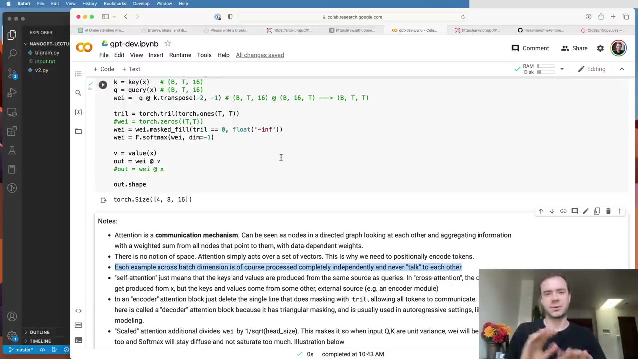
• Batch elements never talk (1:13:23). A batch of 4 with block size 8 is four separate pools of eight nodes.
• Encoder versus decoder blocks (1:14:24). For tasks like sentiment analysis all tokens may talk freely: delete the masking line and you have an encoder block. Keeping the triangular mask makes it a decoder block.
• Self versus cross-attention (1:15:27). It is self-attention because keys, queries and values all come from the same x. In cross-attention the queries come from x while keys and values come from another source, such as an encoder.

1:16:59 – 1:21:37 Scaled attention and the first attention model

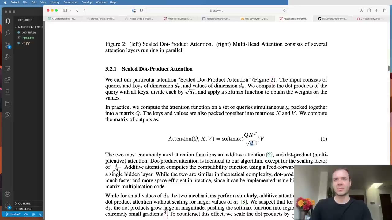
The paper divides scores by √d_k, the head size (1:16:59). Karpathy shows why: with unit-Gaussian q and k, the raw scores have variance around the head size, and the scaling brings it back to about 1. That matters because the scores feed softmax. He demonstrates that multiplying a set of small numbers by 8 makes softmax collapse toward the maximum (1:18:31), meaning each token would draw from a single other token at initialization.

Then he packages it all as a Head module (1:19:03). The triangular mask is stored with register_buffer because it isn’t a trainable parameter. The language model now runs embeddings → one head → lm_head. One more change is needed in generate: because the position table only covers block_size positions, the context is cropped to the last block_size tokens (1:20:34). With a lower learning rate and more iterations, validation loss drops from about 2.5 to 2.4.

1:21:37 – 1:26:49 Multiple heads and a feed-forward layer

Multi-head attention is several heads in parallel with their outputs concatenated (1:21:37). Instead of one 32-dimensional head, four 8-dimensional heads produce 32 channels together; Karpathy likens it to a group convolution. Tokens have many things to look for, so separate channels of communication help: loss falls to about 2.28 (1:23:41).

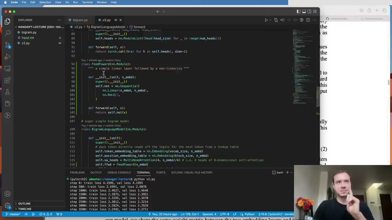
Going back to the paper’s diagram, he points out the feed-forward part (1:24:45). So far tokens gathered information and went straight to the logits, without time to “think” about it. A small per-token MLP, a linear layer followed by ReLU, applied right after attention gives that computation step (1:25:16). Attention is the communication; the feed-forward layer is each token processing what it received on its own. Loss: about 2.24.

1:26:49 – 1:32:33 Blocks and residual connections

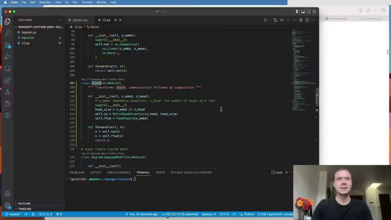
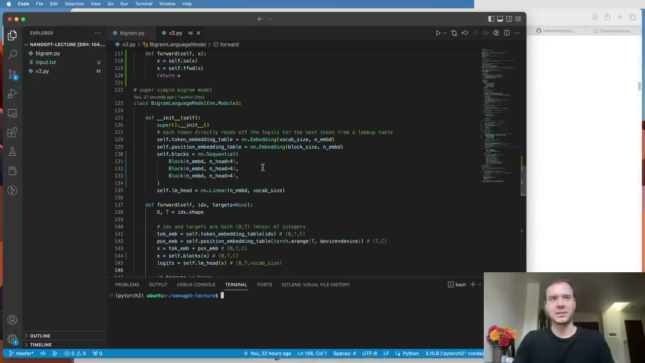
A Block alternates communication and computation: multi-head attention, then feed-forward (1:26:49). The head size is derived as n_embd // n_head, so four heads of 8 for a width of 32. Stacking three blocks, though, makes results worse, because the network is now deep enough to be hard to optimize (1:27:51).

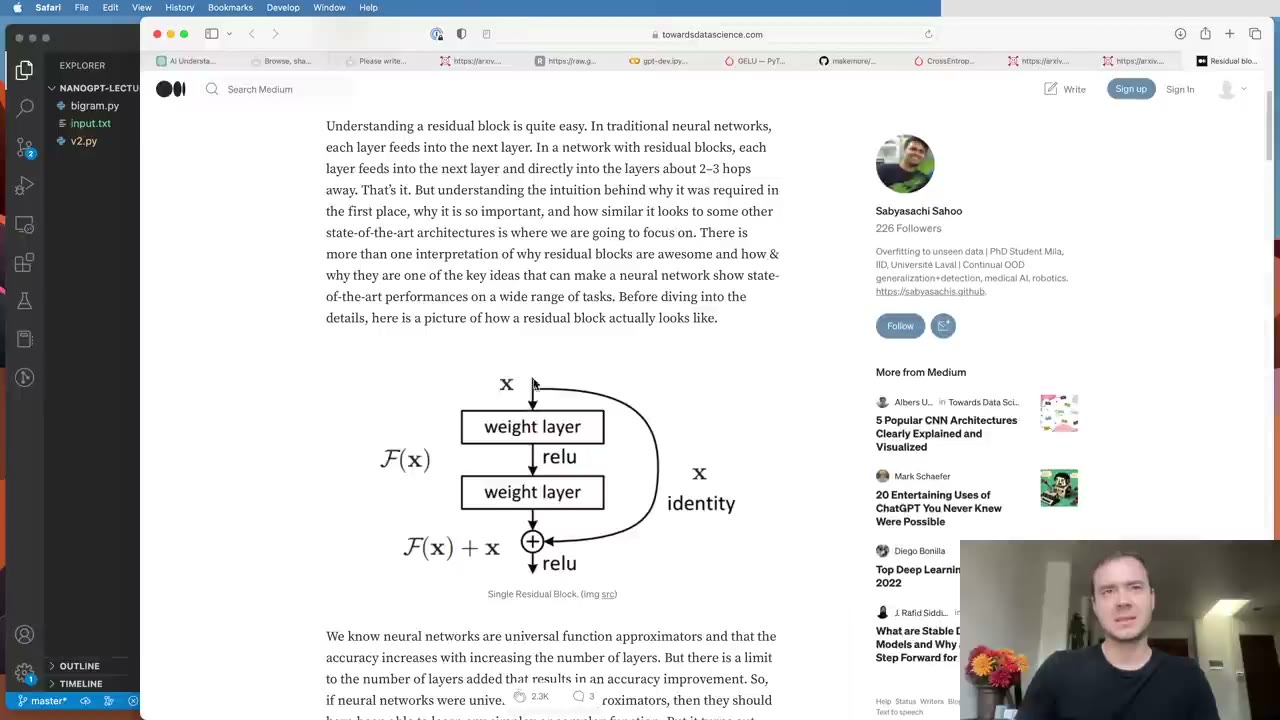
The first fix is residual connections, from the 2015 ResNet paper (1:28:23). Karpathy’s picture is a residual pathway running from input to output, with each block forking off, computing something and adding it back. Since addition passes gradients through unchanged, as seen in micrograd, the loss gradient travels straight to the input, and blocks that contribute little at initialization can come online gradually (1:29:25). In code that is x = x + self.sa(x) and x = x + self.ffwd(x), plus a projection layer at the end of each branch before it rejoins the pathway (1:30:29).

He also follows the paper in making the feed-forward layer’s inner width four times n_embd (1:31:32). Loss reaches 2.08, and for the first time training loss pulls ahead of validation loss, a first sign of overfitting.

1:32:33 – 1:37:47 LayerNorm and the pre-norm layout

The second fix is layer normalization (1:32:33). Karpathy pastes in the BatchNorm1d from the makemore series, which normalizes each column (each feature across the batch), and changes it to normalize each row (each example’s feature vector) instead (1:34:06). Because examples no longer interact, the running buffers and the train/eval distinction disappear. The learnable gamma and beta stay.

He then uses PyTorch’s nn.LayerNorm, with one deviation from the paper: the norm is applied before each sub-layer rather than after, the pre-norm formulation that has become more common (1:35:08). Each block gets ln1 and ln2, normalizing over the 32 features of each token. Loss improves slightly to 2.06, and he adds a final LayerNorm, ln_f, before the output layer (1:37:17). With that, the decoder-only Transformer is essentially complete.

1:37:47 – 1:42:32 Scaling up with dropout

Cosmetic refactors add n_layer and n_head hyperparameters (1:37:47). Dropout goes in three places: on the attention weights after softmax, after the multi-head projection, and at the end of the feed-forward branch (1:38:17). Karpathy describes dropout, from a 2014 paper, as training a random sub-network each step and merging the ensemble at test time; here it is just regularization against the overfitting a bigger model will bring.

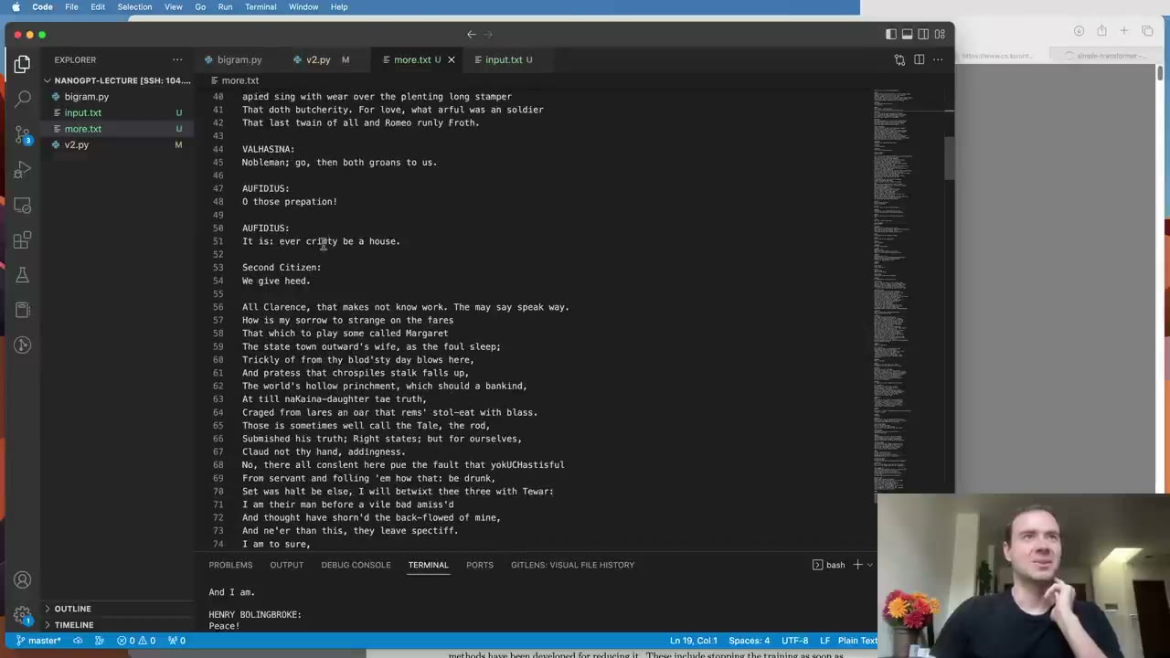
The new settings (1:39:20): batch size 64, block_size 256, a lower learning rate, n_embd 384, 6 heads of 64 dimensions, 6 layers and dropout 0.2. After about 15 minutes on an A100, validation loss is 1.48 (1:40:21). He warns against running this on a CPU or MacBook without shrinking the model. The samples now have the shape of the source, speaker names followed by lines of verse, while remaining nonsense when read (1:41:24).

Our note: the final gpt.py in ng-video-lecture also sets a custom weight initialization (normal with standard deviation 0.02). A comment in the code says it wasn’t covered in this video.

1:42:32 – 1:46:12 Why our model is decoder-only

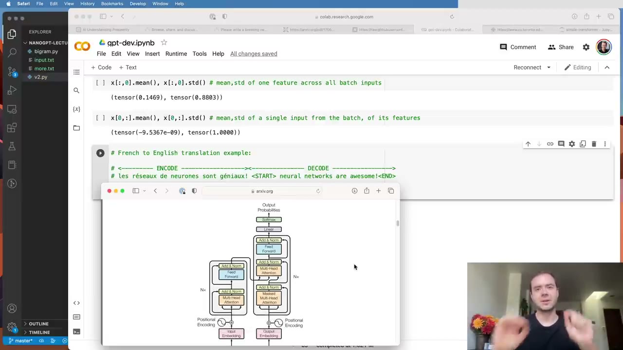
The paper’s diagram has a whole extra column, and Karpathy explains it (1:42:32). What was built is decoder-only: there is no encoder, and no cross-attention sub-layer in the block. It is a decoder because of the triangular mask, which makes it autoregressive and lets it sample text.

The original paper did translation (1:43:34). An encoder reads the French sentence with no mask, so all its tokens talk freely. The decoder generates English from a special start token to an end token, and in every block it reads the encoder’s output through cross-attention: queries come from the decoder, keys and values from the encoder (1:45:07). With nothing to condition on, a GPT doesn’t need that machinery.

1:46:12 – 1:48:44 A tour of nanoGPT

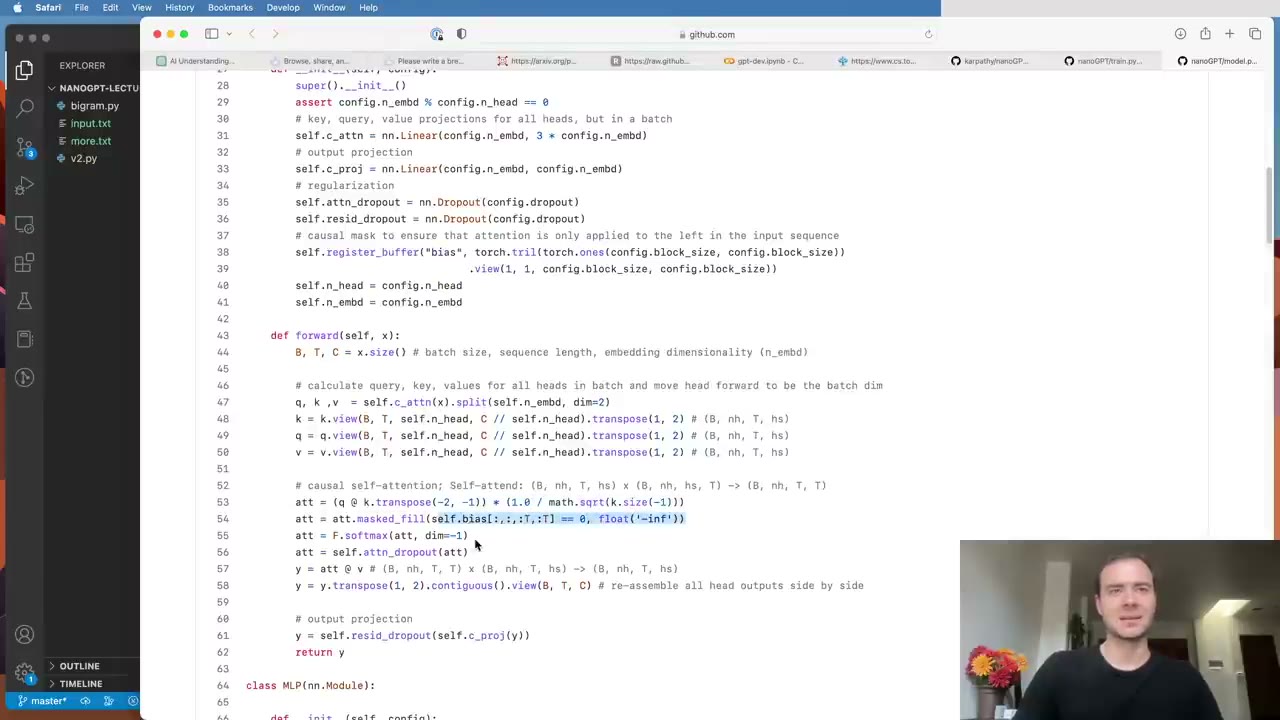
nanoGPT has two files of interest (1:46:12). train.py is the same loop with production extras: checkpoints, pretrained weights, learning-rate decay, model compilation and distributed training. model.py should look familiar. The main difference is that CausalSelfAttention computes all heads at once, treating heads as an extra batch dimension in four-dimensional tensors (1:47:13), which is mathematically the same as the lecture’s list of heads but more efficient. The MLP uses GELU instead of ReLU so OpenAI’s GPT-2 checkpoints can be loaded, and parameters are split into those that get weight decay and those that don’t (1:47:43).

Our note: current nanoGPT also calls PyTorch’s built-in scaled_dot_product_attention (flash attention) when it is available, falling back to the explicit masked softmax shown in the lecture.

1:48:44 – end From pretraining to ChatGPT

Training ChatGPT has two stages (1:48:44). Pretraining is what this lecture did, at a vastly larger scale. Karpathy’s model has about 10 million parameters and saw roughly 300,000 tokens’ worth of text, if counted in OpenAI’s subword vocabulary; the largest GPT-3 has 175 billion parameters trained on 300 billion tokens (1:50:20), with nearly the same architecture and familiar hyperparameters. The difference is scale and infrastructure: thousands of GPUs.

A pretrained model is a document completer (1:51:22). Ask it a question and it may answer with more questions, or carry on as if writing a news article. The second stage aligns it as an assistant, following OpenAI’s ChatGPT blog post (1:52:25): fine-tune on perhaps thousands of question-and-answer documents, have raters rank sampled responses to train a reward model, then optimize the model against that reward with PPO, a policy-gradient reinforcement learning method. Most of that data is private, which makes this stage much harder to reproduce. nanoGPT covers only pretraining.

He closes by recapping (1:54:32): a decoder-only Transformer following the 2017 paper, about 200 lines of training code, released with its commit history and the Colab notebook.

Code you’ll write

These are short excerpts from the finished code. The full scripts, bigram.py and gpt.py, are in karpathy/ng-video-lecture (MIT license), and the production version of the model is model.py in karpathy/nanoGPT.

1. Character tokenizer, splits and batches. Maps each of the 65 characters to an integer, keeps 90% for training, and samples random windows with targets shifted by one. Built from 9:53 to 18:42.

chars = sorted(list(set(text)))
vocab_size = len(chars)
stoi = { ch:i for i,ch in enumerate(chars) }
itos = { i:ch for i,ch in enumerate(chars) }
encode = lambda s: [stoi[c] for c in s]
decode = lambda l: ''.join([itos[i] for i in l])

data = torch.tensor(encode(text), dtype=torch.long)
n = int(0.9*len(data))
train_data, val_data = data[:n], data[n:]

def get_batch(split):
    data = train_data if split == 'train' else val_data
    ix = torch.randint(len(data) - block_size, (batch_size,))
    x = torch.stack([data[i:i+block_size] for i in ix])
    y = torch.stack([data[i+1:i+block_size+1] for i in ix])
    return x.to(device), y.to(device)

2. The bigram model’s forward pass. Each token reads its next-character logits from a table; the reshape lets F.cross_entropy accept them. Built at 22:53, fixed at 26:35.

class BigramLanguageModel(nn.Module):

    def __init__(self, vocab_size):
        super().__init__()
        self.token_embedding_table = nn.Embedding(vocab_size, vocab_size)

    def forward(self, idx, targets=None):
        logits = self.token_embedding_table(idx) # (B,T,C)
        if targets is None:
            loss = None
        else:
            B, T, C = logits.shape
            logits = logits.view(B*T, C)
            targets = targets.view(B*T)
            loss = F.cross_entropy(logits, targets)
        return logits, loss

3. Sampling. Crops the context to block_size, takes the last position’s logits, samples the next index and appends it. Written at 29:11; the crop is added at 1:20:34.

def generate(self, idx, max_new_tokens):
    for _ in range(max_new_tokens):
        idx_cond = idx[:, -block_size:]
        logits, loss = self(idx_cond)
        logits = logits[:, -1, :] # (B, C)
        probs = F.softmax(logits, dim=-1)
        idx_next = torch.multinomial(probs, num_samples=1) # (B, 1)
        idx = torch.cat((idx, idx_next), dim=1) # (B, T+1)
    return idx

4. The masked-softmax averaging trick. Builds a (T, T) matrix whose row t averages positions 0 to t, then applies it to every batch element at once. Shown at 54:33.

tril = torch.tril(torch.ones(T, T))
wei = torch.zeros((T, T))
wei = wei.masked_fill(tril == 0, float('-inf'))
wei = F.softmax(wei, dim=-1)
xbow3 = wei @ x # (T, T) @ (B, T, C) -> (B, T, C)

5. One head of self-attention. Queries and keys set data-dependent affinities, scaled and causally masked; values are what get aggregated. Assembled at 1:19:03.

class Head(nn.Module):

    def __init__(self, head_size):
        super().__init__()
        self.key = nn.Linear(n_embd, head_size, bias=False)
        self.query = nn.Linear(n_embd, head_size, bias=False)
        self.value = nn.Linear(n_embd, head_size, bias=False)
        self.register_buffer('tril', torch.tril(torch.ones(block_size, block_size)))
        self.dropout = nn.Dropout(dropout)

    def forward(self, x):
        B,T,C = x.shape
        k = self.key(x)   # (B,T,hs)
        q = self.query(x) # (B,T,hs)
        wei = q @ k.transpose(-2,-1) * k.shape[-1]**-0.5 # (B,T,T)
        wei = wei.masked_fill(self.tril[:T, :T] == 0, float('-inf'))
        wei = F.softmax(wei, dim=-1)
        wei = self.dropout(wei)
        return wei @ self.value(x) # (B,T,hs)

Our note: in the lecture the scale is typed as C**-0.5, where C is the input width n_embd, not the head size. With a single head of size n_embd the two are equal, but once heads are split (four heads of 8 on a width of 32) it scales by 1/√32 instead of 1/√8. The repository fixed this a week after the video (commit “scale by head size”), and the excerpt above follows the fixed code.

6. Multi-head attention and the Transformer block. Heads run in parallel and are concatenated and projected; the block wraps attention and the feed-forward layer in pre-norm residual connections. Built between 1:21:37 and 1:35:08.

class MultiHeadAttention(nn.Module):
    def __init__(self, num_heads, head_size):
        super().__init__()
        self.heads = nn.ModuleList([Head(head_size) for _ in range(num_heads)])
        self.proj = nn.Linear(head_size * num_heads, n_embd)
        self.dropout = nn.Dropout(dropout)
    def forward(self, x):
        out = torch.cat([h(x) for h in self.heads], dim=-1)
        return self.dropout(self.proj(out))

class Block(nn.Module):
    def __init__(self, n_embd, n_head):
        super().__init__()
        head_size = n_embd // n_head
        self.sa = MultiHeadAttention(n_head, head_size)
        self.ffwd = FeedFoward(n_embd) # Linear(n_embd, 4*n_embd), ReLU, Linear back, Dropout
        self.ln1 = nn.LayerNorm(n_embd)
        self.ln2 = nn.LayerNorm(n_embd)
    def forward(self, x):
        x = x + self.sa(self.ln1(x))
        x = x + self.ffwd(self.ln2(x))
        return x

FeedFoward is spelled that way in the repository. The full model, GPTLanguageModel (still named BigramLanguageModel on screen in the video), adds token and position embeddings, n_layer blocks in an nn.Sequential, the final ln_f and lm_head.

Skip list

• 0:02 – 3:10 ChatGPT demos and the paper’s background. Skip if you know what a language model does.
• 21:51 – 37:50 The bigram model, loss, sampling and training loop, repeated quickly from makemore. Skim it, but keep the cross-entropy reshape at 26:35 and the generate design note at 34:05.
• 37:50 – 41:59 Converting the notebook into a script. Skip unless you plan to run bigram.py yourself.
• 47:10 – 50:23 The 3×3 matrix-multiplication walk-through. Skip if you already see why a lower-triangular matrix of ones produces running sums.
• 1:33:04 – 1:35:08 Rewriting BatchNorm as LayerNorm. Skip if you remember BatchNorm from Lecture 4 and only want the result.
• 1:48:44 – end ChatGPT’s training stages. Conceptual only, with no code; skip if you came for the implementation.

Glossary

• Language model — a model that assigns probabilities to what comes next in a sequence; generating text means sampling from it repeatedly.
• Token / tokenizer — the units a model reads and the scheme that converts text into integers for them; here single characters, in GPT subword pieces.
• Vocabulary size — the number of distinct tokens; 65 for Tiny Shakespeare’s characters, about 50,000 for GPT-2’s encoding.
• block_size (context length) — the maximum number of past tokens the model sees when predicting the next one.
• Batch dimension — independent sequences stacked into one tensor so a GPU can process them together; they never exchange information.
• Logits — the unnormalized scores for each possible next token; softmax turns them into probabilities.
• Cross-entropy loss — the negative log probability the model gave to the correct next token, averaged over all positions.
• Bigram model — a language model that predicts the next token from the current token alone.
• Embedding table — a learned lookup table that turns a token or position index into a vector.
• Position embedding — a learned vector for each position in the context, added to the token embedding so attention can tell positions apart.
• Self-attention — a layer in which each token builds a weighted average of other tokens’ values, with weights computed from its query and their keys.
• Query, key, value — three linear projections of each token: what it seeks, what it offers to be matched on, and what it passes along when chosen.
• Head / head_size — one independent attention computation and the width of its queries, keys and values.
• Causal mask — the lower-triangular mask that stops a position from attending to later positions, making the model autoregressive.
• Scaled dot-product attention — attention whose scores are divided by the square root of the head size, keeping softmax from saturating at initialization.
• Multi-head attention — several heads run in parallel on narrower slices, with outputs concatenated and projected back to the model width.
• Feed-forward layer — a small per-token MLP, here 4× wider inside, that processes what attention gathered.
• Residual connection — adding a block’s output back to its input, which gives gradients a direct path through deep networks.
• LayerNorm — normalization of each token’s feature vector to zero mean and unit variance, followed by a learned scale and shift.
• Pre-norm — applying LayerNorm before each attention and feed-forward sub-layer instead of after, as the original paper did.
• Dropout — randomly zeroing a fraction of activations during training to reduce overfitting.
• Decoder-only Transformer — a Transformer of masked self-attention blocks with no encoder, the GPT design.
• Cross-attention — attention whose queries come from one sequence and whose keys and values come from another, such as an encoder’s output.
• Pretraining / fine-tuning — training a document completer on a huge text corpus, then adapting it to act as an assistant with curated examples and reward-model reinforcement learning.

Studying another course? Paste its YouTube or Bilibili link on the home page to request a handout — or make your own with the desktop app (coming soon).