3Blue1Brown neural networks ch. 1: what is a neural network? — notes

Updated 2026-10-02 · Video: 3Blue1Brown, published 2017-10-05 · 19 min

9 key slides

Watch the video (19 min)

Watch the original video on YouTube

Chapter 1 of 3Blue1Brown’s neural networks series builds a plain “multilayer perceptron” that reads a 28×28 handwritten digit and guesses which digit it is. It covers only the structure: what the neurons hold, how one layer computes the next, and why the whole thing is one big function. Learning is left to chapter 2 on gradient descent. You need no machine learning background; comfort with a weighted sum and a little matrix-vector multiplication helps. The course overview is on the 3Blue1Brown neural networks index.

Key takeaways

A neuron is a number between 0 and 1. The input layer has 784 of them, one per pixel; the output layer has 10, one per digit (2:37).
Layers are motivated by a hope, not a guarantee: pixels might combine into edges, edges into loops and lines, and those into digits (5:49). Chapter 2 shows the trained network does not actually do this.
Each neuron computes sigmoid(weighted sum + bias). Weights pick the pixel pattern, the bias sets the threshold (8:41).
The network has 13,002 knobs. “Learning” means finding good values for all of them (12:14).
One layer to the next is a = σ(Wa + b). Writing it as a matrix-vector product makes the math compact and the code fast (13:32).
Sigmoid is a teaching choice. Modern deep networks mostly use ReLU because it trains more easily (17:16).

Chapter notes

0:00 – 2:37 Why recognising a “3” is hard

The video opens on a sloppy, low-resolution 3. People read it instantly, yet writing a program that does the same thing by hand is very hard, because two images of a 3 can share almost no pixel values. That gap is the reason to want a system that learns from examples instead of following hand-written rules.

Grant Sanderson limits the series to the simplest network type, with no convolutions or other modern additions. He calls this “a necessary prerequisite” for the more powerful variants. That is a fair framing. Convolutional nets, LSTMs and transformers all reuse the same building block shown here: a weighted sum, a bias and a nonlinearity.

2:37 – 5:39 Neurons, activations and layers

The definition is deliberately bare: “a thing that holds a number, specifically a number between 0 and 1.” That number is the neuron’s activation. The first layer has 784 neurons, one per pixel of the 28×28 image, with 0 for black and 1 for white. The last layer has 10 neurons, and the brightest one is the network’s answer. In between are two hidden layers of 16 neurons each. Grant admits both numbers are arbitrary: two layers suit his story, and 16 fits on screen.

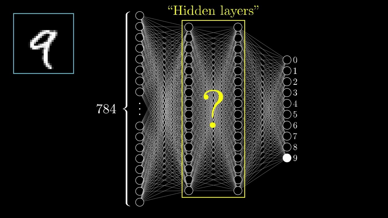
Network diagram with a 784-neuron input column, two hidden layers marked with a yellow question mark and the label Hidden layers, and a 10-neuron output column, next to a handwritten 9 — 4:33 — The full architecture: 784 inputs, two hidden layers of 16, and 10 outputs. The question mark is honest. At this point nothing explains what the hidden layers should compute.

The key mechanical idea is that activations in one layer fully determine the activations in the next. Feed in an image and a pattern of brightness flows forward, layer by layer, until one output neuron is brightest. This one-way flow is called the forward pass. Keep it in mind, because backpropagation runs the same graph in reverse.

5:39 – 8:21 Why layers might help: edges, loops, digits

Here Grant gives the motivation for stacking layers. People recognise digits by their parts. A 9 is a loop on top plus a line on the right, an 8 is two loops, a 4 is a few strokes. If the second-to-last layer had one neuron per part, the last layer would only need to learn which parts make which digit.

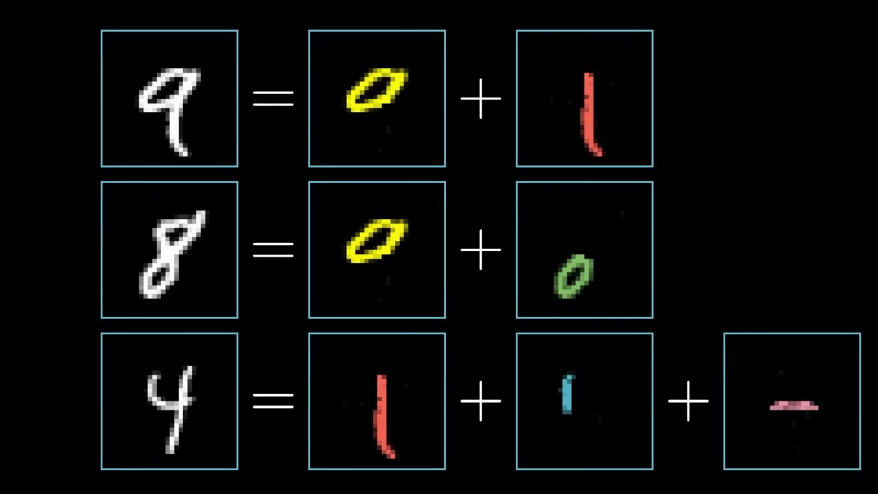
Digits broken into parts: 9 equals an upper loop plus a vertical line, 8 equals two loops, 4 equals three separate strokes — 6:04 — The decomposition that motivates the hidden layers. Each part on the right is what one third-layer neuron would ideally detect.

The same trick applies one level down. A loop is a ring of small edges, and a long line is a row of edges. So the hope is that layer 2 detects little edges, layer 3 detects loops and lines, and layer 4 detects digits.

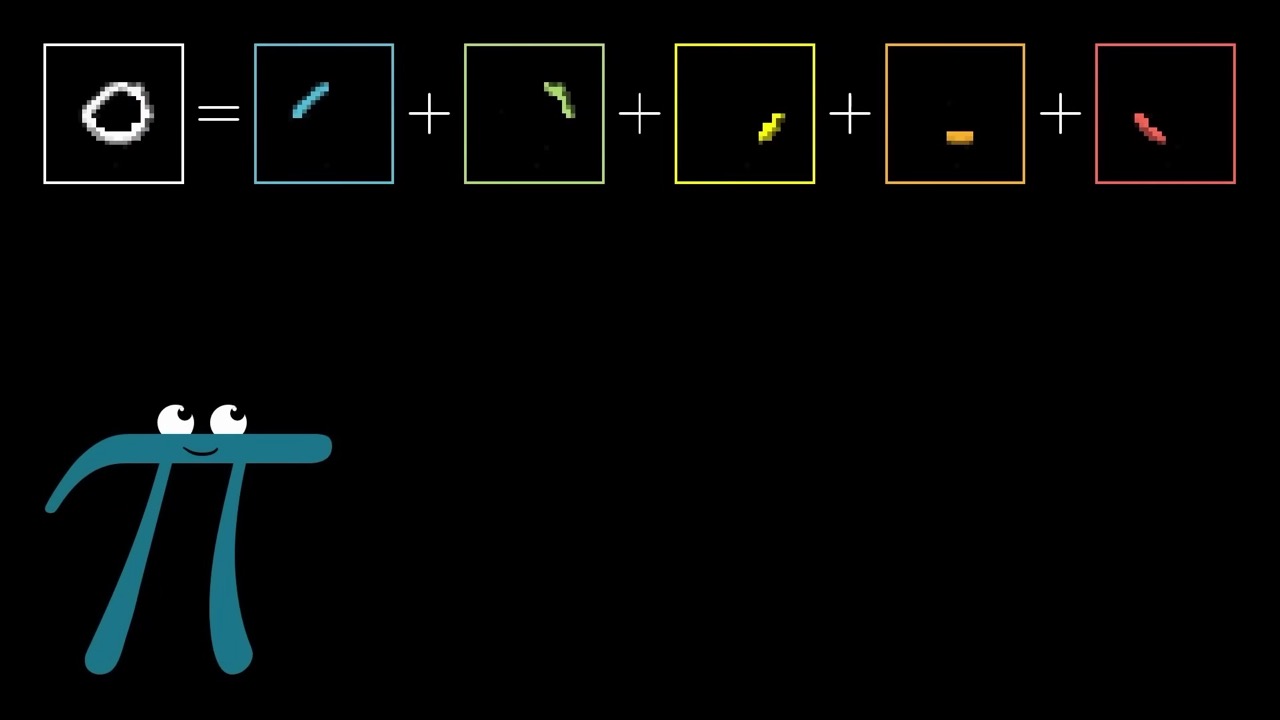
A loop shape shown as the sum of five small edge segments in different orientations — 7:02 — A loop written as a sum of short edges. This is the "little edge" layer idea: each hidden-layer-1 neuron fires for one edge in one place.

Treat this section as a design hypothesis. Grant says plainly that whether the trained network does this is “another question.” In chapter 2 at 14:02 he shows the learned weights, and they look nothing like clean edges. The broader point holds, though: many tasks, from vision to speech, break into layers of abstraction, and that is why depth helps in practice.

8:21 – 11:43 Weights, the sigmoid and the bias

To make one second-layer neuron detect one edge, give it a weight for each of the 784 input pixels and compute the weighted sum. Picture the weights as their own 28×28 grid, green for positive and red for negative. Positive weights in a small strip and negative weights around it make the sum large only when the strip is bright and its surroundings are dark. That is an edge detector.

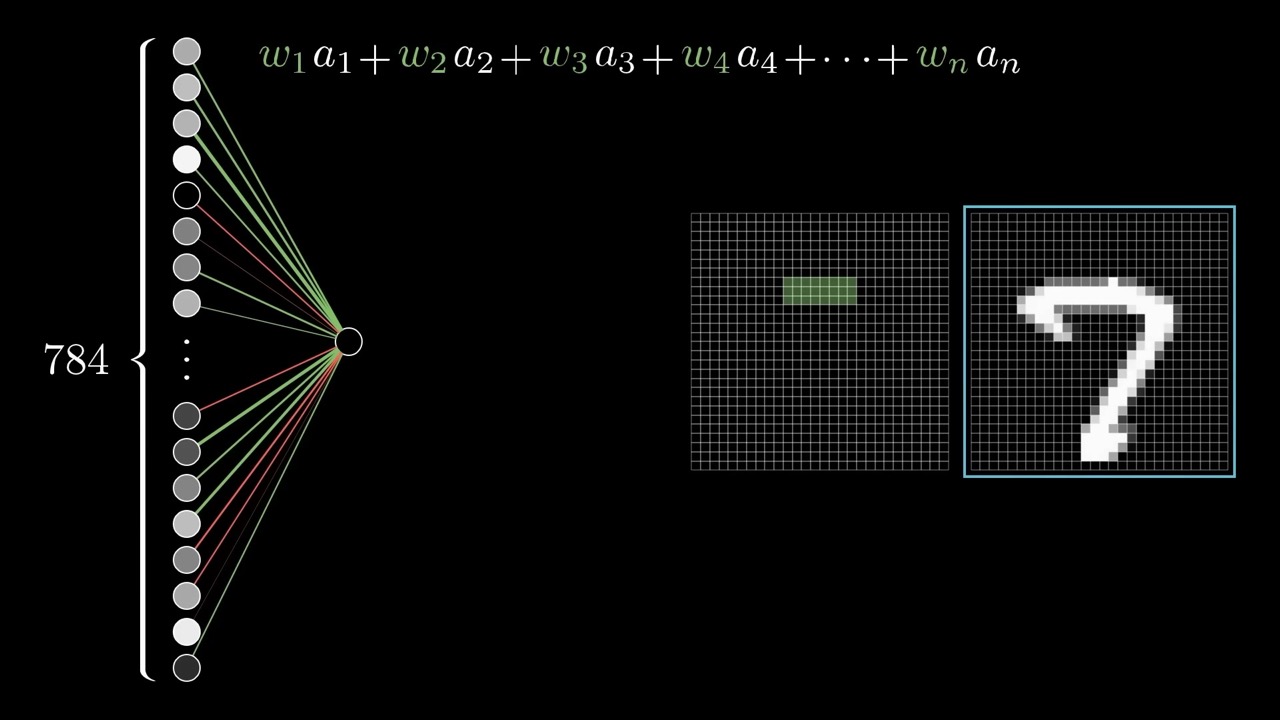
Weighted sum w1a1 + w2a2 + ... + wnan from 784 input neurons into one neuron, with the weight grid shown as a green strip beside a handwritten 7 — 9:49 — The weights drawn as an image. Only pixels under the green strip contribute, so the sum measures how bright that one region is.

A weighted sum can be any real number, but this network wants activations between 0 and 1. So the sum is passed through the sigmoid (logistic) function, which squashes very negative inputs toward 0 and very positive ones toward 1. A bias is added first, for example −10, so the neuron only lights up once the sum clearly exceeds 10.

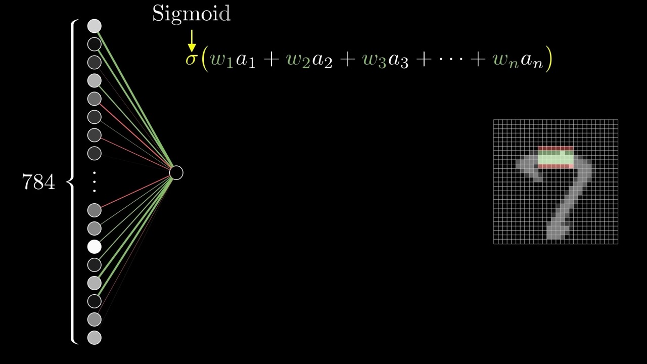
Formula sigmoid of w1a1 + w2a2 + ... + wnan minus 10, labelled bias, with the note: only activate meaningfully when weighted sum is greater than 10 — 10:49 — The full single-neuron rule: σ(weighted sum + bias). The weights decide what pattern the neuron looks for; the bias decides how strong the evidence must be.

A useful way to remember the split of roles: weights are a template, the bias is a threshold. Both are just numbers the network will learn.

11:43 – 13:32 Counting the knobs

Every one of the 16 second-layer neurons has its own 784 weights and one bias. The same holds between every pair of layers. The slide shows the total.

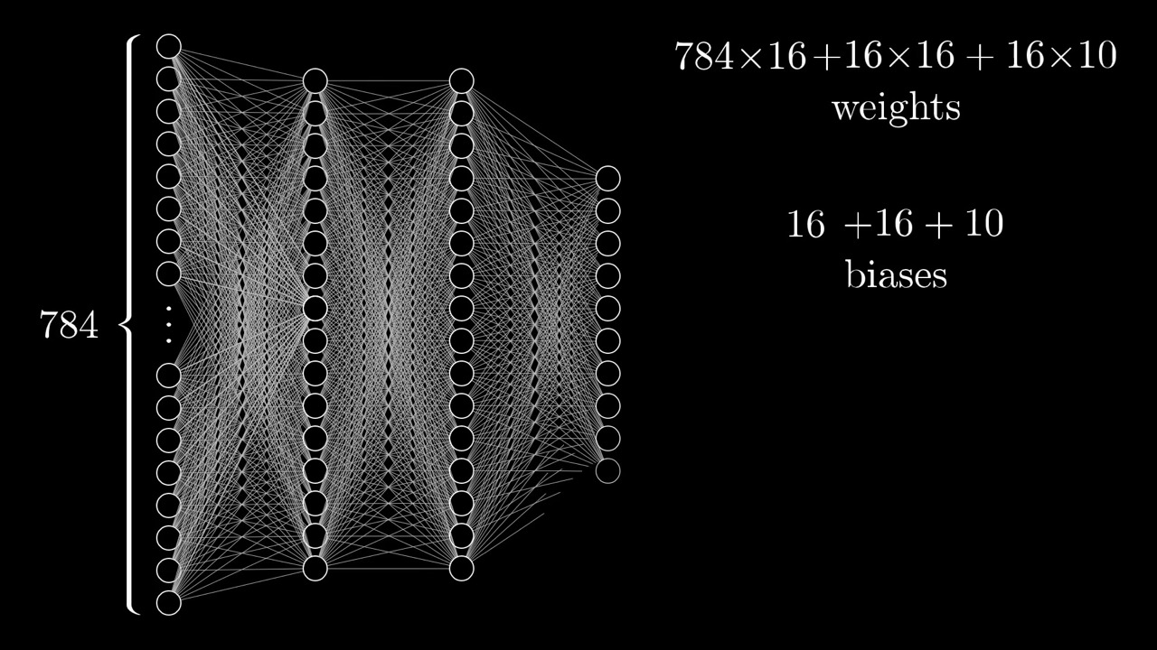
Fully connected network with the box 784×16 + 16×16 + 16×10 weights and 16 + 16 + 10 biases, totalling 13,002 — 12:14 — 12,960 weights plus 42 biases gives 13,002 parameters. Almost all of them sit between the input and the first hidden layer.

The arithmetic is worth doing yourself: 784×16 = 12,544, so the first connection layer holds over 96% of all parameters. That is typical. Input-facing layers in fully connected networks are expensive, which is one reason convolutional networks share weights across the image. In the video “learning” is defined simply as finding a setting of these 13,002 numbers that solves the task. Grant also argues for thinking about what the weights mean rather than treating the network as a black box. It gives you somewhere to start when it fails.

13:32 – 15:18 The matrix form

Writing every neuron out by hand gets messy, so the video packs one layer transition into one expression. Put the previous layer’s activations in a column vector a. Put the weights in a matrix W, one row per neuron in the next layer. Then each entry of Wa is one neuron’s weighted sum. Add a bias vector b and apply σ to each entry.

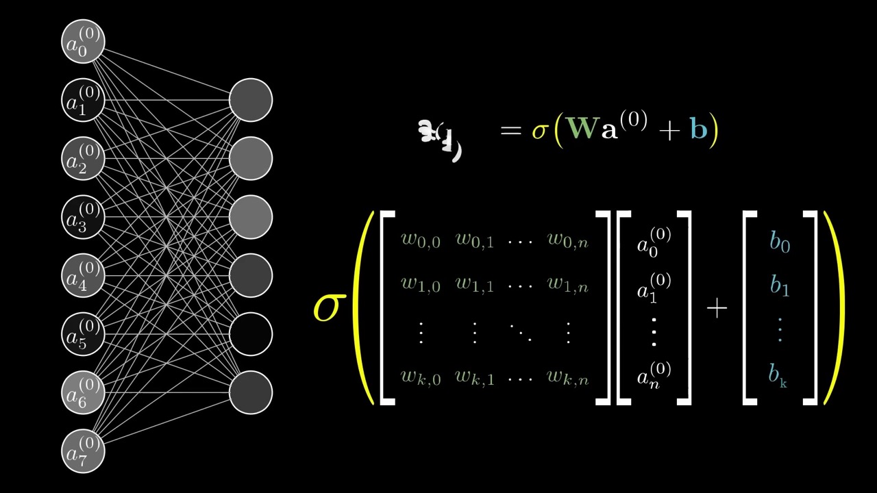
Expression a(1) = σ(W a(0) + b) written out with the full weight matrix, activation vector and bias vector — 15:03 — a⁽¹⁾ = σ(Wa⁽⁰⁾ + b). This line is the whole layer. It is also what the code computes, and fast matrix libraries are why it runs quickly.

A common pitfall: row j of W holds the weights into neuron j. Chapter 4 keeps that convention when it writes w_jk, so it is worth fixing now. If matrix-vector products feel shaky, Grant points to chapter 3 of his linear algebra series.

15:18 – 16:23 The network is just a function

Grant now refines the earlier definition. A neuron does not just hold a number. It is a function of the previous layer’s outputs. Scale that up and the entire network is a function from 784 numbers to 10 numbers, built from repeated matrix-vector products and sigmoids, with 13,002 parameters.

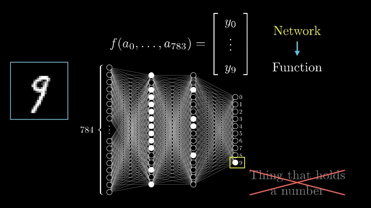
f(a0, ..., a783) = (y0, ..., y9) written beside the network, with Network → Function and the phrase Thing that holds a number crossed out — 15:41 — The key reframe: "thing that holds a number" is crossed out and replaced with "function." Chapter 2 builds a second function, the cost, on top of this one.

This reframe is what makes the rest of the series possible. Once the network is a differentiable function of its parameters, calculus can tell you how to adjust them. That is the subject of gradient descent and backpropagation calculus.

16:23 – 18:40 Outro and the ReLU aside

After the subscribe joke and Patreon thanks, Grant talks briefly with Lisha Li, a deep learning PhD at Amplify Partners. She says few modern networks still use sigmoid. ReLU, the rectified linear unit max(0, a), is “much easier to train” for very deep networks.

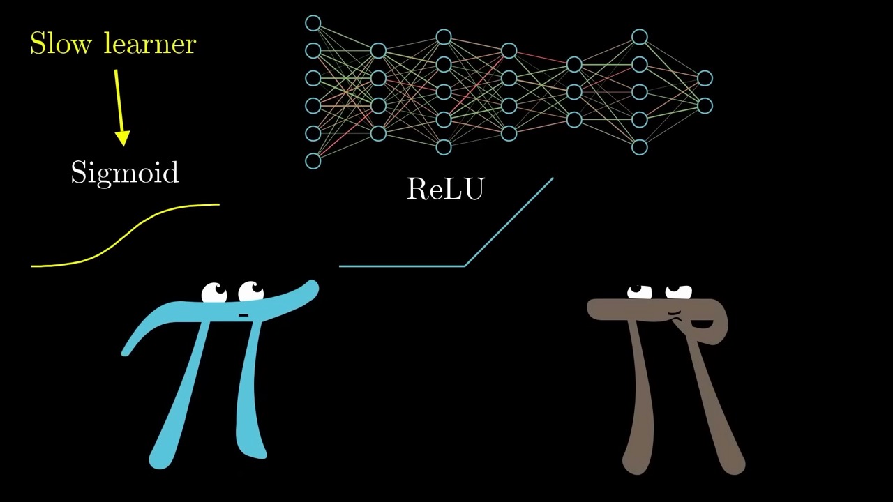
Sketch comparing a sigmoid curve labelled slow learner with a ReLU curve that is flat at zero and then rises linearly — 18:18 — Sigmoid ("slow learner") versus ReLU. Everything in this chapter works the same with ReLU; only the squashing function changes.

Our note: the reason ReLU trains better is linked to gradients. A sigmoid flattens out at both ends, so its derivative is tiny there, and those tiny factors multiply across layers during backpropagation. You can see exactly where that factor appears in the σ′(z) term of chapter 4.

Skip list

1:10 – 2:07 Motivation for why machine learning matters. Skip it if you already know why you are here.
8:01 – 8:21 The speech-recognition analogy. It repeats the idea of layered abstraction.
12:43 – 13:32 The “set the weights by hand” thought experiment. Worth hearing once; no new mechanics.
16:23 – 17:16 Subscribe and Patreon segment.

Glossary

Activation — the number a neuron currently holds; here between 0 and 1.
Hidden layer — any layer between input and output; its meaning is learned, not designed.
Weight — a number on each connection that scales the previous neuron’s activation in the weighted sum.
Bias — a number added to the weighted sum that shifts the neuron’s activation threshold.
Sigmoid (logistic function) — σ(x) = 1 / (1 + e⁻ˣ); squashes any real number into (0, 1).
ReLU — rectified linear unit, max(0, x); the default nonlinearity in most modern networks.
Multilayer perceptron — a plain fully connected feed-forward network like the one in this video.
MNIST — the standard dataset of labelled 28×28 handwritten digits used throughout chapters 1–3.

FAQ

What is a neuron in 3Blue1Brown's neural network video?

In this video a neuron is just a thing that holds a number between 0 and 1, called its activation. Later in the video it is reframed as a function: it takes all activations of the previous layer and returns one number.

Why does the network in the video have 13,002 parameters?

The network has layers of 784, 16, 16 and 10 neurons. That gives 784×16 + 16×16 + 16×10 = 12,960 weights plus 16 + 16 + 10 = 42 biases, for 13,002 numbers that training must set.

What does the bias do in a neuron?

The bias is added to the weighted sum before the sigmoid. It sets how large the weighted sum must be before the neuron becomes meaningfully active, like a threshold.

Do modern networks still use the sigmoid function?

Mostly not. In the interview at the end, Lisha Li notes that ReLU, max(0, a), turned out much easier to train for deep networks, so sigmoid is now considered old school for hidden layers.

Studying another course? Paste its YouTube or Bilibili link on the home page to request a handout — or make your own with the desktop app (coming soon).