3Blue1Brown neural networks ch. 3: backpropagation intuition — notes
Watch the video (13 min)
Watch the original video on YouTube
Chapter 3 walks through backpropagation without formulas. It follows one training image, a handwritten 2, and asks what that image “wants” from every weight, bias and neuron, working backwards from the output. Then it averages those wishes over many examples and introduces mini-batch stochastic gradient descent. You should know the network from chapter 1 and the cost and gradient from chapter 2. The same ideas in calculus form come next in chapter 4.
Key takeaways
- Read the gradient as sensitivities. An entry of 3.2 versus 0.1 means the cost is 32 times more sensitive to the first weight (1:27).
- One example’s wishes are proportional to its errors. Output neurons far from their target get the biggest nudges (3:56).
- Three levers per neuron: bias, weights (in proportion to the previous activation) and previous activations (in proportion to the weight) (4:42).
- “Backwards” means summing every output neuron’s wishes for the layer before, then repeating (7:35).
- Average over examples, but in mini-batches. This is stochastic gradient descent: noisier steps, much faster progress (9:19).
Chapter notes
0:00 – 2:42 Recap, and the gradient as sensitivity
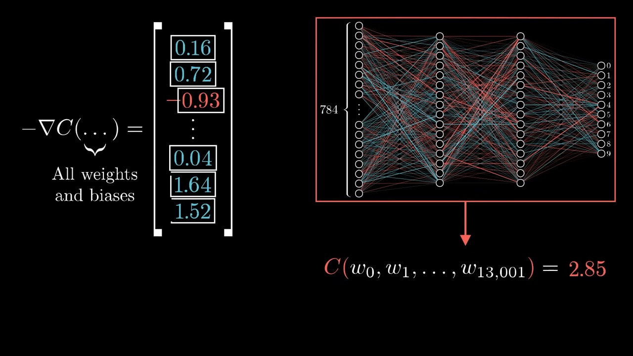
After recapping the 784-16-16-10 network and the squared-error cost, Grant sets up the one idea to hold onto. A 13,002-dimensional direction is impossible to picture. Instead, read each gradient entry as how sensitive the cost is to that one parameter.
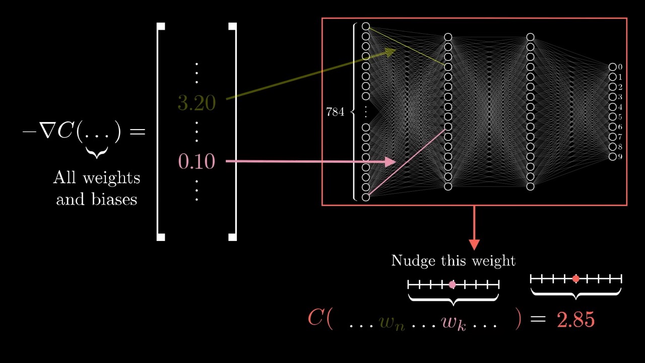
He also admits what makes backprop feel hard: “the notation and the index chasing.” Each step is simple. The difficulty is that many small effects are layered on top of each other. That is why this chapter postpones notation entirely.
2:42 – 3:56 Focus on a single example
The true cost averages over all training data, so in principle every example affects every step. To understand the mechanics, Grant looks at one image of a 2 and asks how that example alone would like the weights and biases to change.
3:56 – 5:55 What the output layer wants, and three ways to get it
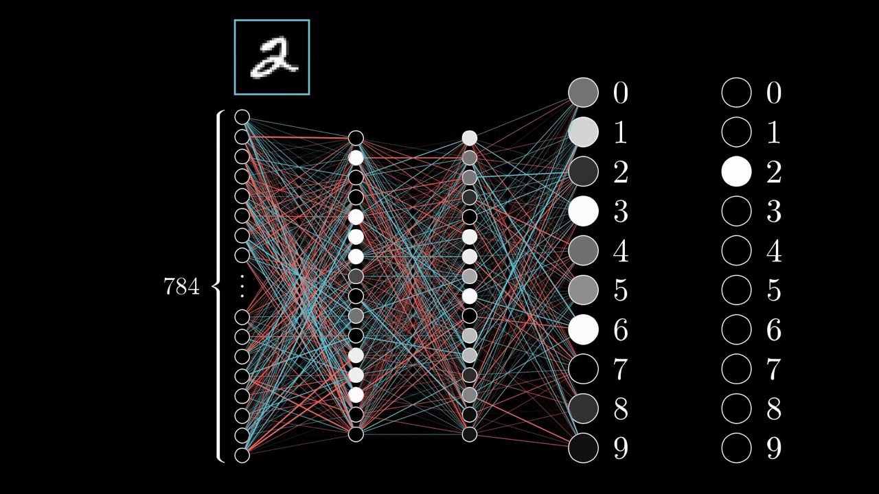
The untrained network gives scattered outputs like 0.5, 0.8, 0.2. We want the “2” neuron to go up and the other nine to go down, each in proportion to how far it is from its target. A neuron already near 0 barely needs attention; one at 0.8 that should be 0 needs a lot.
Zoom in on the “2” neuron. Its activation is σ(w₀a₀ + … + wₙ₋₁aₙ₋₁ + b), so there are three ways to raise it.
The proportionality is the point. A weight is multiplied by its input activation, so raising a weight on a bright input buys far more than raising one on a dim input. That is exactly the “bang for your buck” ranking from chapter 2.
5:55 – 6:38 “Fire together, wire together”
Grant notes a loose parallel with Hebbian theory in neuroscience. The largest weight increases happen between neurons that are already active and the neuron we want more active. Those firing while seeing a 2 get linked more strongly to the neuron that represents 2.
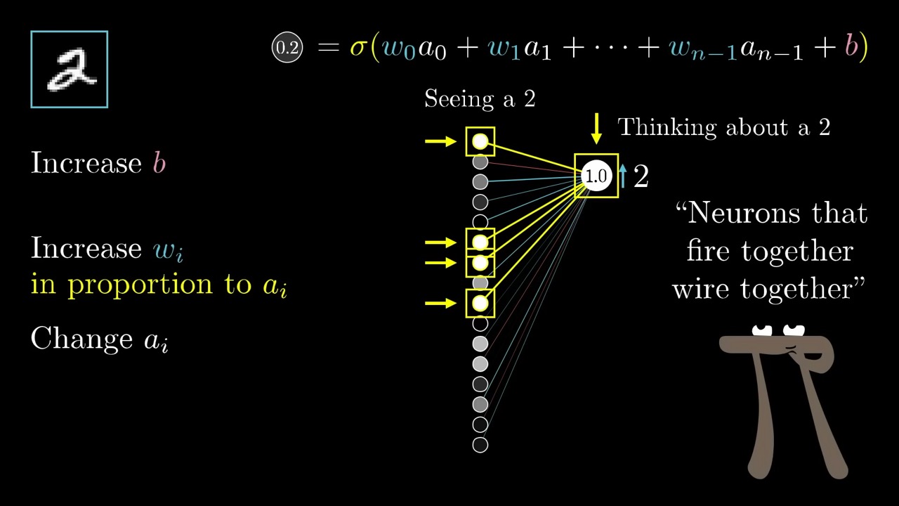
He is careful to call this “a very loose analogy” and not a claim about brains. We would add one caveat. In the real update, weights can also decrease, for connections into neurons that should be dimmer. “Fire together, wire together” describes only half of what backprop does.
6:38 – 8:45 Wishes for the previous layer, and why it runs backwards
The third lever is changing the previous layer. If every neuron with a positive weight into “2” got brighter and every one with a negative weight got dimmer, “2” would rise. Again the payoff scales with the size of each weight. We cannot set those activations directly, but we can record what we wish they were.
The crucial step comes next. The “2” neuron is not the only one with opinions about the previous layer. All nine other output neurons want to go down, and each has its own wishes for the same 16 neurons.
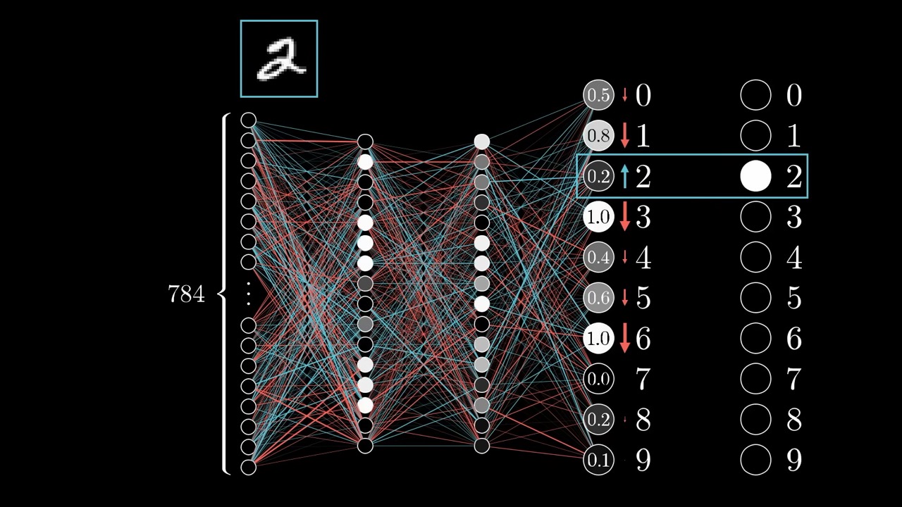
Summing those wishes gives a list of desired nudges for the second-to-last layer. Now that layer looks exactly like the output layer did a minute ago: neurons with targets. So you apply the same reasoning to its weights and biases, and keep going.
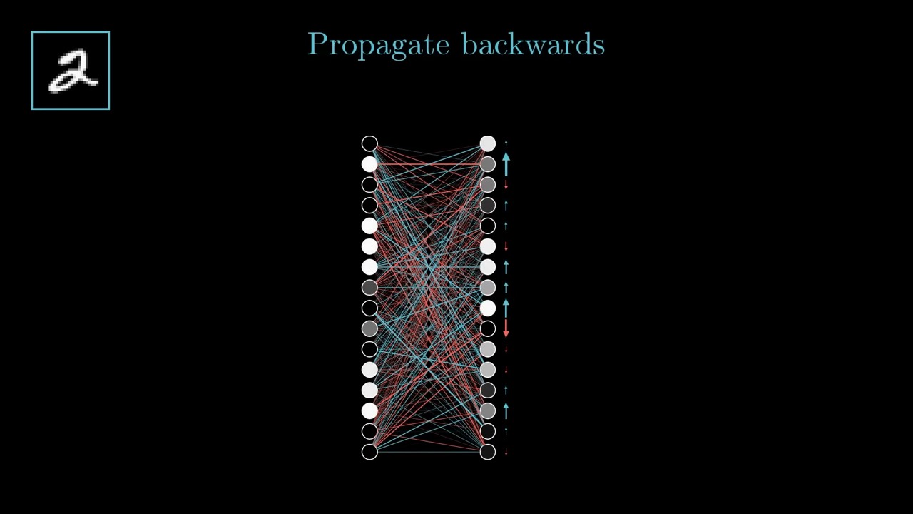
This is the core insight, and it is mainly about efficiency. You compute each layer’s “desired change” once and reuse it for every weight feeding into that layer. You never trace each weight’s effect all the way to the cost separately. Chapter 4 shows that this “desired change” is the derivative of the cost with respect to an activation.
8:45 – 9:52 Averaging over all training examples
If you listened only to the 2, the network would learn to call everything a 2. So run the same routine for every training example, record each one’s desired nudges to every parameter, and average them.
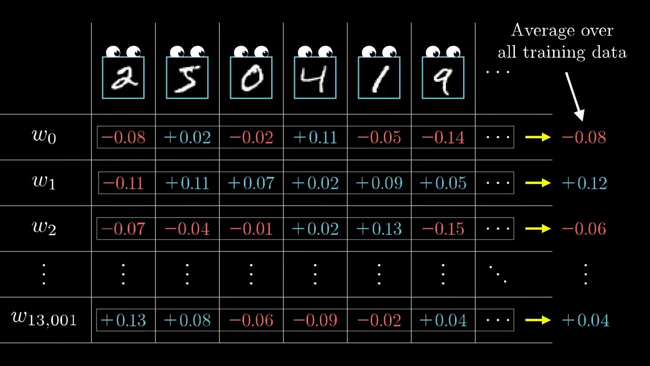
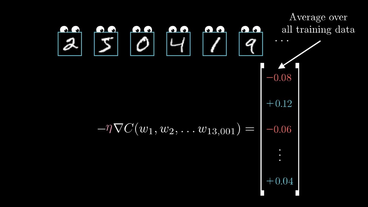
Grant says “loosely speaking” because he has not yet made the nudges quantitatively exact. That is chapter 4’s job.
9:52 – 11:33 Mini-batches and stochastic gradient descent
Running backprop on every training example for every step is slow. The standard fix is to shuffle the data, cut it into mini-batches of, say, 100 examples, and take one step per mini-batch.
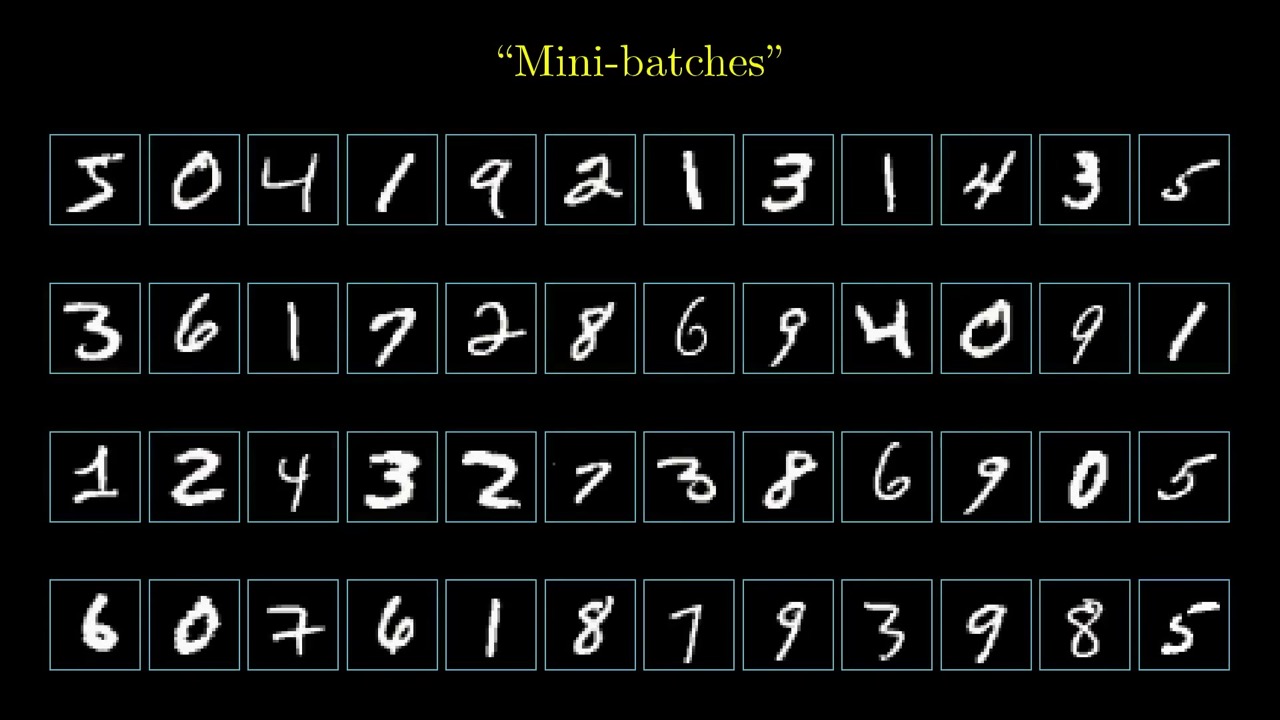
Grant’s image: “a drunk man stumbling aimlessly down a hill but taking quick steps” rather than a careful walker computing the exact downhill direction. This is stochastic gradient descent (SGD). The trade-off is worth stating plainly. Each step points roughly downhill rather than exactly, but you can take many more steps for the same compute.
11:33 – 12:47 Summary and the data problem
Grant’s summary: backprop tells you how one example wants to nudge each parameter, in relative proportions. True gradient descent averages over all examples, and SGD approximates that with mini-batches. Every line of a backprop implementation corresponds to something shown in this chapter. He ends on a practical point: all of this needs a lot of labelled data, which MNIST supplies for digits but most real problems do not.
Skip list
- 0:09 – 1:27 Plan and recap of chapters 1–2. Skip it if you are watching in order.
- 6:25 – 6:38 Disclaimer about neuroscience. It is short and adds no new idea.
- 10:41 – 11:33 Spoken summary of the chapter. It is useful as review but covered above.
Glossary
- Backpropagation — the algorithm that computes the gradient of the cost by passing desired changes from the output layer back toward the input.
- Desired nudge — informal name for how much one example wants a parameter or activation to change; formally a partial derivative.
- Hebbian theory — the neuroscience idea that “neurons that fire together wire together.”
- Mini-batch — a small random subset of the training data used to estimate the gradient for one step.
- Stochastic gradient descent (SGD) — gradient descent where each step uses a mini-batch instead of the full dataset.
- η (eta) — the learning rate, the scale factor on the gradient for each step.
FAQ
What is backpropagation in simple terms?
Backpropagation is the algorithm that computes how each weight and bias should change to lower the cost. Starting from what the output layer needs, it works out what each earlier layer should do, layer by layer backwards, and turns those wishes into nudges for every parameter.
What are the three ways to increase one neuron's activation?
Increase its bias, increase its weights (most of all those attached to bright neurons in the previous layer), or change the previous layer's activations in proportion to the weights. Only the first two can be changed directly; the third is passed back to the earlier layer.
Why do we average over training examples?
One example on its own would push the network toward always giving that one answer. Averaging the desired nudges from many examples gives a step that improves the network on all of them, which is, up to scaling, the negative gradient.
What is stochastic gradient descent?
Instead of averaging over every training example per step, you shuffle the data, split it into mini-batches of, say, 100 examples, and take one step per mini-batch. Each step is less precise but much cheaper.
Studying another course? Paste its YouTube or Bilibili link on the home page to request a handout — or make your own with the desktop app (coming soon).