3Blue1Brown neural networks ch. 2: gradient descent — notes
Watch the video (21 min)
Watch the original video on YouTube
Chapter 2 explains what it means for a neural network to “learn”: define a cost that measures how wrong the network is, then repeatedly nudge all 13,002 weights and biases downhill on that cost. It then tests the trained network and finds it works well while learning something quite different from what chapter 1 hoped for. Watch chapter 1 first. Basic calculus (a slope, a minimum) is enough; multivariable calculus helps but is not required. The next step is backpropagation, intuitively.
Key takeaways
- Learning = minimizing a cost function. The cost takes all weights and biases as input and returns one number for how badly the network does on the training data (2:56).
- Gradient descent steps against the gradient. Compute the direction of steepest increase, step the opposite way, repeat (7:54).
- You only find a local minimum. Where you end up depends on the random starting point (5:52).
- Each gradient entry is an importance score. Its sign says up or down, its size says how much that parameter matters (10:46).
- About 96% test accuracy, but no edge detectors. The learned weights look almost random, and the network is confidently wrong on noise (13:14).
Chapter notes
0:00 – 1:56 Recap of the network
A quick replay of chapter 1: 784 input neurons, two hidden layers of 16, ten outputs, and about 13,000 weights and biases. If chapter 1 is fresh, you can skim this.
1:56 – 3:05 Training data, test data and MNIST
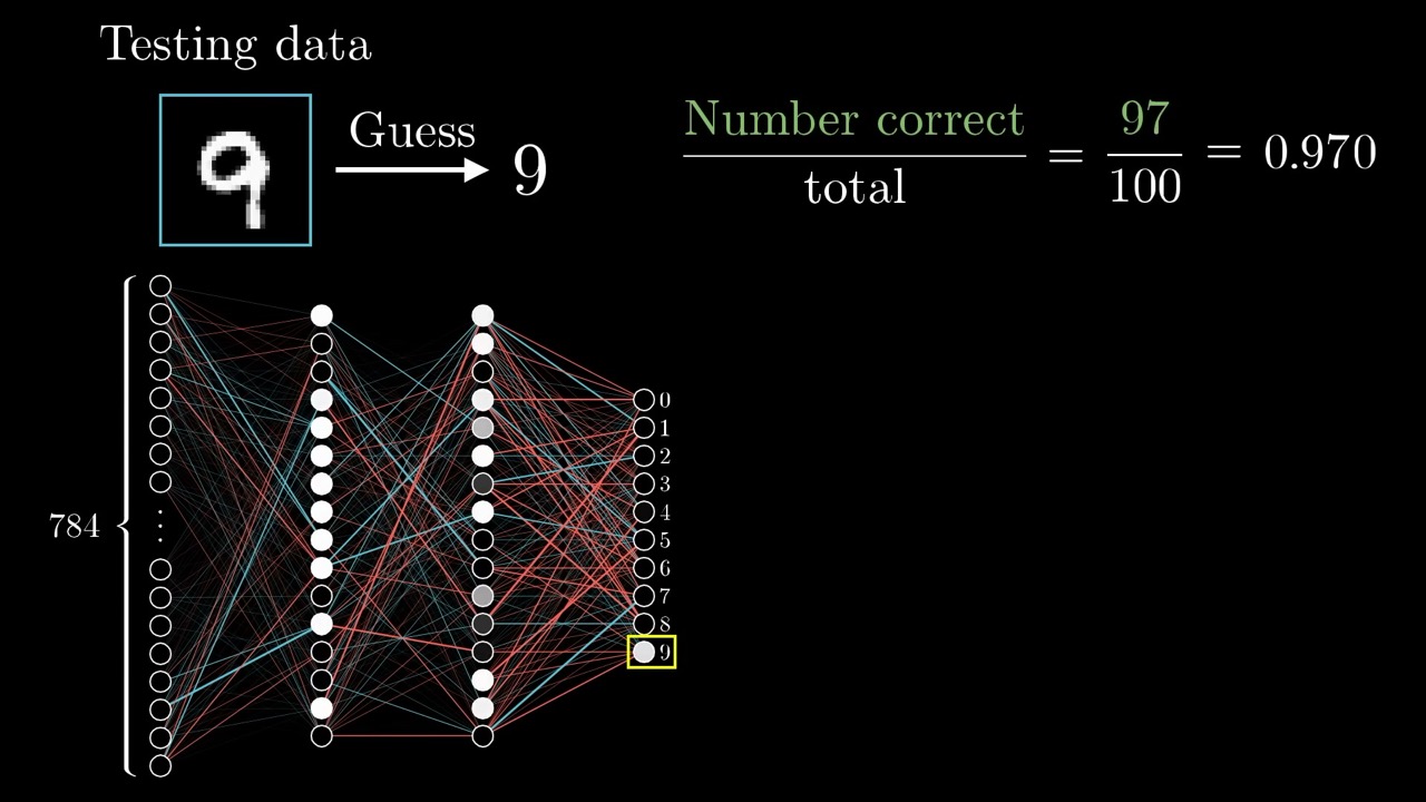
The setup for learning is labelled examples: images of digits along with the right answer. Training adjusts the parameters to do well on those images. The real test is images the network has never seen. Grant credits the MNIST database for supplying tens of thousands of labelled digits. He also defuses the hype: learning “feels a lot less like some crazy sci-fi premise, and a lot more like a calculus exercise.”
The distinction between training and test data matters more than the video’s brief mention suggests. A network that scores well on its training images but poorly on new ones has memorized rather than generalized. The research segment at the end returns to exactly this problem.
3:05 – 5:12 The cost function
Start with random weights and the network outputs noise. To tell it how wrong it is, compare its 10 outputs with the target (1 for the right digit, 0 for the rest) and add up the squared differences. That is the cost of one example. Average it over every training example and you get the cost of the whole network.
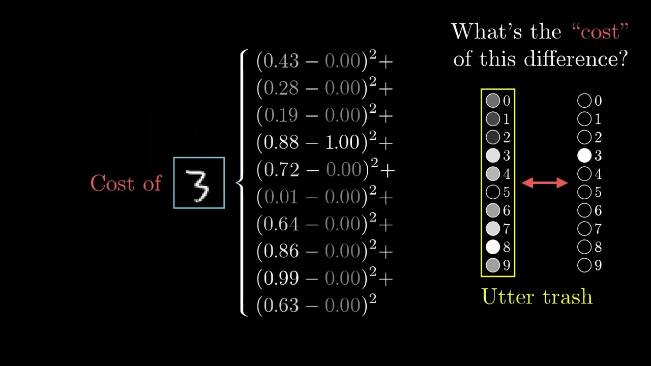
The important shift is what the cost is a function of. The network maps pixels to outputs. The cost maps parameters to a single score, with the training data held fixed.
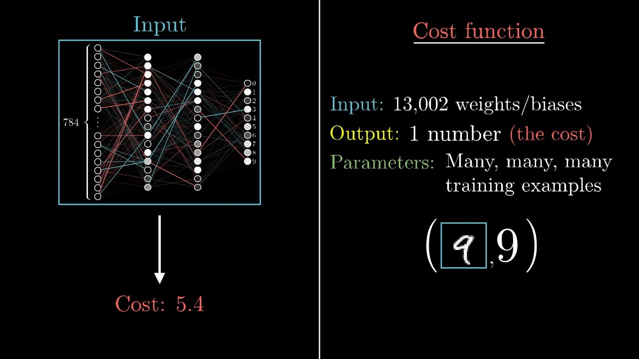
Note that squared error is the choice for this teaching example. Classifiers in practice usually use cross-entropy on softmax outputs instead, but the descent idea is the same.
5:12 – 7:54 Rolling downhill
To build intuition, shrink the problem to one input. You cannot always solve for the minimum directly, so start somewhere, check the slope, and step left if it is positive or right if it is negative. Keep going and you settle into a valley, like a ball rolling downhill.
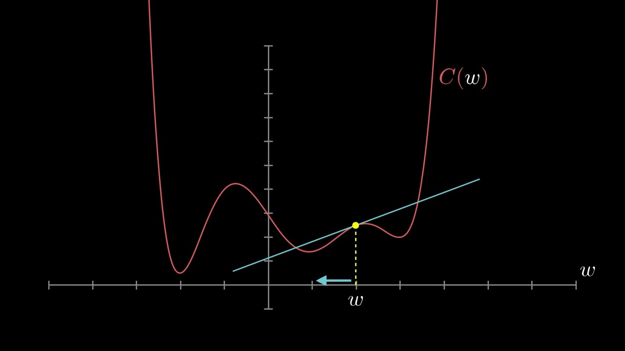
Two details carry over to real networks. First, you only find a local minimum. Second, if the step size is proportional to the slope, steps shrink as the ground flattens, which helps avoid overshooting. In two dimensions the slope becomes the gradient, the direction of steepest ascent. Its negative points downhill, and its length says how steep the slope is.
7:54 – 10:37 The gradient in 13,002 dimensions
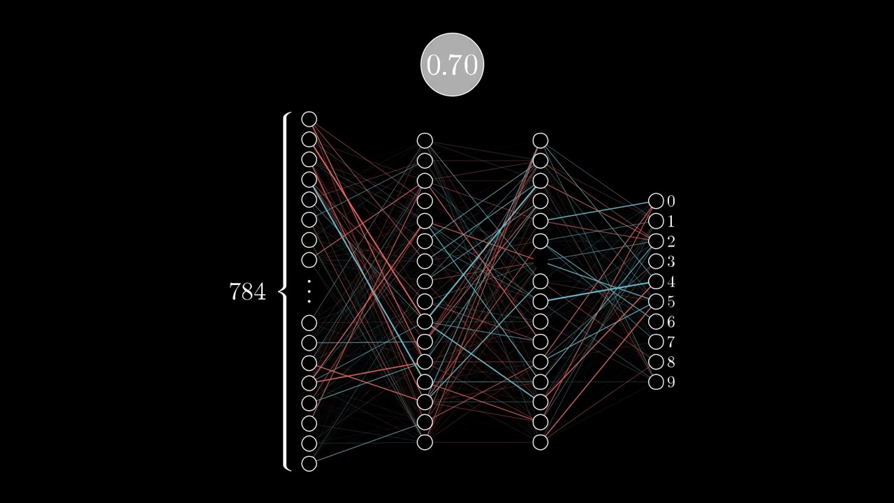
The algorithm does not change with dimension. Stack all 13,002 weights and biases into one column vector. The negative gradient of the cost is another column of the same length, and it tells you which nudge to every parameter lowers the cost fastest.
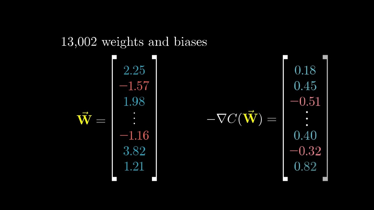
Grant names the algorithm that computes this gradient efficiently: backpropagation, covered in chapter 3 and chapter 4. He also explains a design choice from chapter 1. Artificial neurons have continuous activations, not on/off states like biological neurons, because the cost must be smooth for small downhill steps to work.
10:37 – 12:20 The gradient as an importance ranking
Since 13,002 dimensions cannot be visualized, Grant offers a non-spatial reading. The sign of each gradient component says up or down. The relative magnitudes say which changes matter most. Some connections simply have more influence on the cost for this training data.
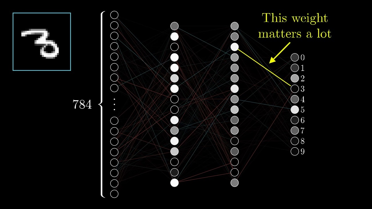
His two-variable example makes this concrete. If the gradient at a point is (3, 1), then nudging x matters three times as much as nudging y near that point. We find this reading the most useful one for the next two chapters. Backpropagation is easiest to follow as bookkeeping for these sensitivities.
12:20 – 13:06 Three layers of complexity
A compact summary worth writing down. The network is a function of 784 pixels. The cost is a function of 13,002 parameters, built on top of the network. The gradient of the cost is a third layer: it tells you how to change those parameters.
13:06 – 16:46 How well does it work, and what did it learn?
Trained this way, the network classifies about 96% of new images correctly, and about 98% after some tweaks to the hidden layers.
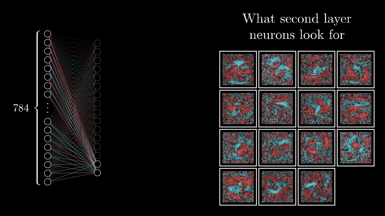
Then comes the twist. Visualize the weights into each second-layer neuron the same way as in chapter 1, and instead of neat edges you get noise with loose blobs in the middle. In Grant’s words, the network settled into “a happy little local minimum” that classifies well without learning the hoped-for parts.
A second test drives it home. Feed in random noise and the network does not hedge. It confidently picks a digit.
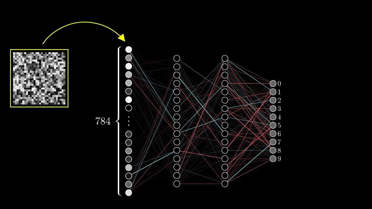
Grant’s explanation is the training setup itself. The network only ever saw centred, clean digits, and the cost never rewarded anything but confidence. That is the real lesson of this section. A network optimizes exactly what the cost measures on exactly the data it sees, and nothing more. He calls this 1980s–90s technology, a starting point before modern variants.
16:46 – 17:40 Where to learn more
Grant asks viewers to pause and think how they would change the system to better detect edges. He recommends Michael Nielsen’s free online book Neural Networks and Deep Learning, which has code for this exact example, plus Chris Olah’s blog and Distill articles.
17:40 – 19:59 Research corner: memorization or structure?
Lisha Li describes a paper in which a deep image network was trained on shuffled, meaningless labels and still reached the same training accuracy as on real labels. That raises the question of whether minimizing cost is learning structure or just memorizing. A later paper she mentions found a difference in how fast the cost falls.
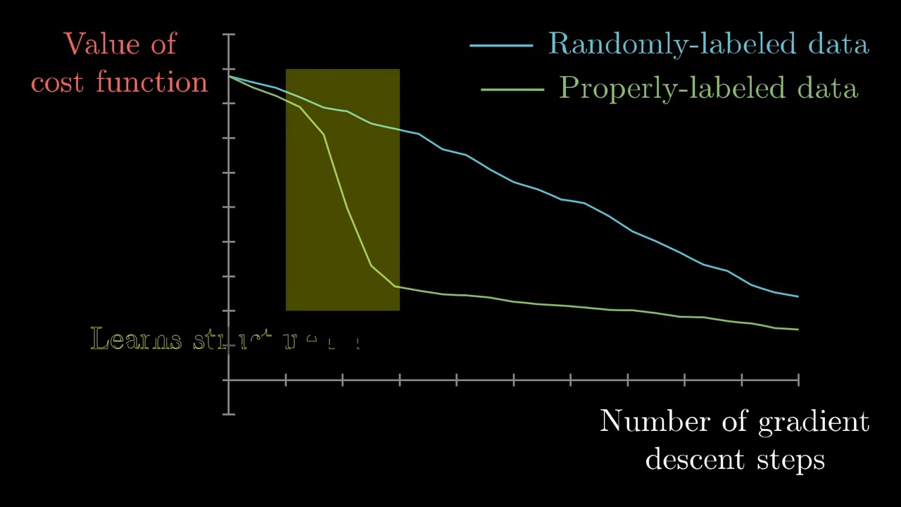
She closes with an older result: for networks under simplifying assumptions, the local minima tend to be of roughly equal quality. That partly answers the worry from 5:52 about getting stuck in a bad valley. The paper names are not given in the video, so we do not cite them here.
Skip list
- 0:00 – 1:56 Recap of chapter 1. Skip it if you just watched it.
- 7:54 – 8:39 Khan Academy plug and reassurance about multivariable calculus.
- 16:13 – 17:40 “Pause and ponder” prompt and resource list. The resources are listed above.
- 19:59 – 20:33 Patreon and sponsor thanks.
Glossary
- Cost function (loss) — a single number measuring how badly the network performs on the training data, as a function of its parameters.
- Gradient — the vector of partial derivatives of the cost; it points in the direction of steepest increase.
- Gradient descent — repeatedly moving parameters by a small multiple of the negative gradient.
- Local minimum — a valley in the cost surface that is not necessarily the lowest point overall.
- Training set / test set — labelled data used to fit the parameters, and separate data used to check generalization.
- Generalization — performing well on inputs the network never saw during training.
- Learning rate — the multiple of the gradient used for each step; the video calls it a “small multiple.”
FAQ
What is the cost function in 3Blue1Brown's gradient descent video?
For one image, it is the sum of squared differences between the 10 output activations and the desired output (1 for the correct digit, 0 elsewhere). The full cost averages this over all training examples, so it is a function of the network's 13,002 weights and biases.
What does the negative gradient tell you?
It is a vector with one entry per weight and bias. The sign of each entry says whether that parameter should go up or down, and its relative size says how much that change matters for lowering the cost.
How accurate is the simple network in the video?
With two hidden layers of 16 neurons it classifies about 96% of unseen test images correctly. With some tweaks to the hidden layers, the video says it reaches about 98%.
Does the trained network detect edges and loops as hoped?
No. When the video visualises the weights into the first hidden layer, they look almost random, and the network confidently labels pure noise as a digit. It found a local minimum that works without learning the hoped-for structure.
Studying another course? Paste its YouTube or Bilibili link on the home page to request a handout — or make your own with the desktop app (coming soon).