3Blue1Brown neural networks: how AI images and video work — notes

Updated 2026-10-02 · Video: 3Blue1Brown, published 2025-07-25 · 37 min

10 key slides

Watch the video (37 min)

Watch the original video on YouTube

This is a guest video on the 3Blue1Brown channel, presented by Stephen Welch of Welch Labs; Grant Sanderson speaks only at the end, to introduce him. It explains how text-to-image and text-to-video models work in three parts: CLIP, which links text and images in one vector space; diffusion, viewed as Brownian motion run backwards; and guidance, which steers diffusion toward a prompt. It is the longest video in the playlist and the least dependent on the others. Embeddings and cosine similarity from the transformers chapter help, and the idea of a model as learned weights trained by gradient descent is assumed.

Key takeaways

Generation starts from random noise. A transformer repeatedly turns a pure-noise video into something realistic; Wan 2.1 uses 50 steps (1:20).
CLIP learns a shared space for images and text by pulling matching pairs together and pushing non-matching pairs apart, so you can do arithmetic on concepts (5:02).
Diffusion models learn a time-dependent vector field that points noisy points back toward the data, and predicting the total noise is a lower-variance way to learn it (15:21).
Adding noise during sampling prevents blurry averages; DDIM later showed a deterministic method reaches the same final distribution in fewer steps (19:34).
Classifier-free guidance amplifies the prompt’s effect: the difference between prompted and unprompted outputs, scaled by α (33:09).

Chapter notes

0:10 – 3:31 A real model, step by step

Welch starts hands-on with Wan 2.1, an open-source video model. “An astronaut riding a horse on the Moon” gives a convincing clip; an empty prompt still produces a video of a woman. In the source code, generation starts with a call to a random number generator: a video of pure noise. A transformer turns it into a slightly structured video, which is fed back in, 50 times over (1:29).

He frames the whole video around a claim: diffusion is closely tied to the physics of Brownian motion, and that link gives practical algorithms, not just a nice analogy. The three parts are CLIP, diffusion and guidance (2:19).

3:31 – 8:23 CLIP: one space for words and pictures

OpenAI’s CLIP (2021) is two models, a text encoder and an image encoder, trained on 400 million image-caption pairs. Each outputs a vector of length 512.

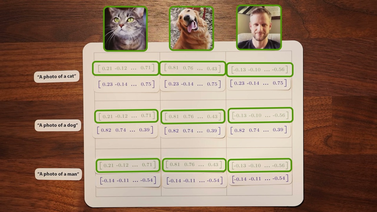
A board with photos of a cat, a dog and a man along the top and captions 'A photo of a cat/dog/man' down the side, each cell pairing an image vector with a text vector; diagonal cells highlighted in green — 5:02 — The contrastive training grid. Diagonal cells are matching image-caption pairs and should have high similarity; every off-diagonal cell should be low. One batch therefore teaches both "what matches" and "what does not".

Similarity is cosine similarity, the cosine of the angle between two vectors, which is 1 when they point the same way (5:44). Compare this with the dot product from the transformers chapter: cosine similarity is a dot product with the lengths divided out.

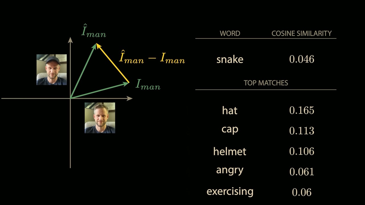
Vector diagram of Welch with and without a hat, the difference vector I_man_hat − I_man, and a table of words by cosine similarity: hat 0.165, cap 0.113, helmet 0.106, angry 0.061, exercising 0.06 — 7:07 — Concept arithmetic in CLIP space: photo with hat minus photo without hat lands nearest the word "hat". It is the image-text version of the king/queen analogy in Chapter 5.

CLIP can classify images zero-shot by comparing an image vector against one caption per label. But it only maps into the shared space; it cannot generate an image from a vector (8:02). That is the gap diffusion fills.

8:23 – 11:39 DDPM and two surprises

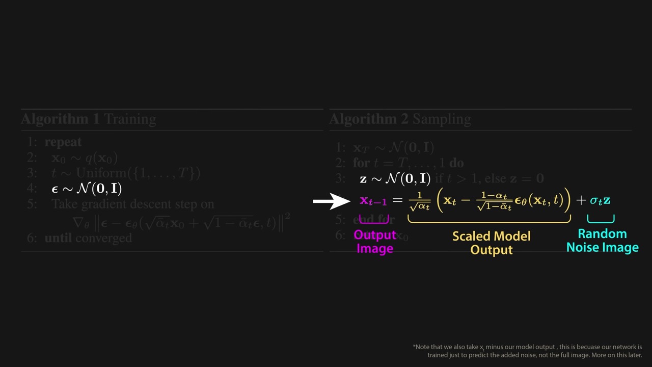
The 2020 Berkeley paper “Denoising Diffusion Probabilistic Models” (DDPM) showed high-quality image generation from noise. The naive picture is to train a network to undo one noise step at a time, then chain it. Welch says virtually no modern model works like that, and points to two surprises in the paper’s algorithms.

DDPM Algorithm 2 (Sampling) with the update line annotated: output image x_{t−1}, scaled model output, plus sigma_t z labelled 'Random Noise Image' — 9:56 — Surprise one: during generation, every step adds fresh random noise (σₜz) after the model's prediction. Surprise two, from Algorithm 1: the model is trained to predict the total noise added to a clean image, not one step's worth.

Two Stable Diffusion outputs for 'A lone tree standing in the middle of a desert': with DDPM sampling a clear tree and dunes; with random steps removed a blurry beige image with a tiny smudge — 10:29 — Remove the noise-adding line and Stable Diffusion 2 gives a "tiny sad blurry tree". The rest of the video explains why.

11:39 – 17:33 Diffusion as a vector field

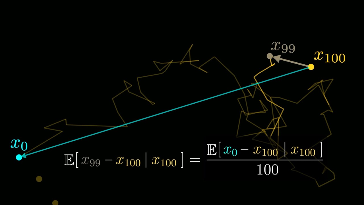
To see what is going on, shrink images to two pixels so each image is a point in 2D, and make the “real images” lie on a spiral. Adding noise to an image is a random step for its point; adding noise repeatedly is a random walk, the Brownian motion that gives diffusion its name (13:17). Generation means running that walk backwards.

Predicting step 99 from step 100 is noisy, because the last step was random. But on average points drift away from the spiral, so a model can still learn to point back.

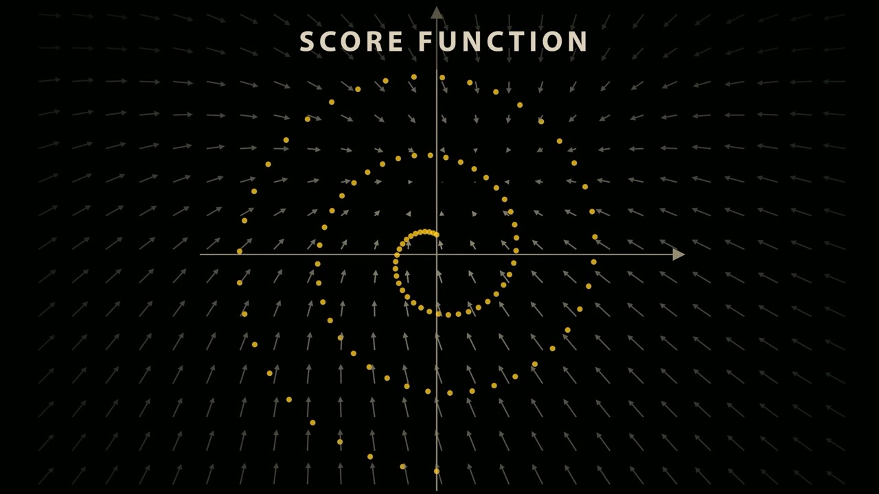
A random walk from x0 to x100 with a cyan line from x100 back to x0, and the equation E[x99 − x100 | x100] = E[x0 − x100 | x100] / 100 — 15:21 — Why DDPM's training target works. The expected last step equals the expected total displacement divided by the number of steps, so predicting the whole way back to x₀ is the same objective with much less noise in each training example.

Vector field labelled SCORE FUNCTION with small arrows over a 2D plane all pointing toward a spiral of yellow points — 16:07 — The learned vector field, also called a score function: at every point, the direction toward more likely, less noisy data.

The right field depends on how noisy the point is: far away it should point roughly at the spiral, close by it should follow the fine structure. So the model also takes a time input t (1 at full noise, near 0 when nearly clean). Watching the trained field over time, around t ≈ 0.4 it switches from pointing at the spiral’s centre to pointing at the spiral itself, which Welch likens to a phase change (17:18).

17:33 – 22:09 Why sampling needs noise

Follow DDPM generation in 2D: step along the field, add a random kick, repeat with shrinking kicks. A cloud of 256 points lands spread along the spiral. Remove the kicks and every point slides to the centre and then to one inside edge (18:53).

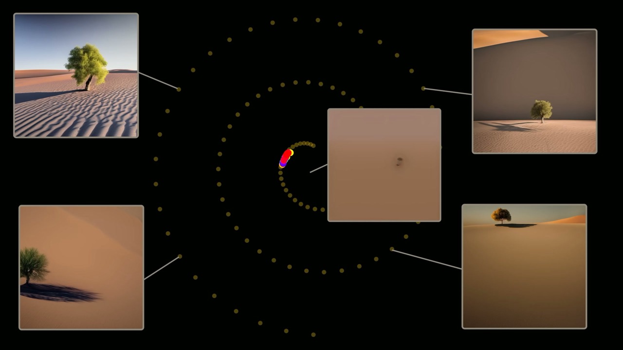
The 2D spiral with four desert-tree images placed at different points on it, and a blurry tree image at the centre where all noise-free samples collapsed — 19:34 — Different points on the spiral stand for different good tree images; their average sits in the middle and looks blurry. Welch notes the 2D analogy is imperfect: in real image space the samples fail to reach realistic images at all.

The theory explains it: for small steps the reverse process is Gaussian, and the model learns its mean. To actually sample rather than return the average, you must add zero-mean Gaussian noise, which is exactly DDPM’s extra line (20:48). This is a general pitfall worth remembering: a model trained to minimise squared error predicts averages, and averages of images are blurry.

22:09 – 24:57 DDIM: same distribution, no randomness

DDPM needs many steps, each a full pass through a large network. Teams at Stanford and Google showed you can drop the random steps. DDPM sampling is a stochastic differential equation; using the Fokker–Planck equation from statistical mechanics, there is an ordinary differential equation with the same final distribution of points.

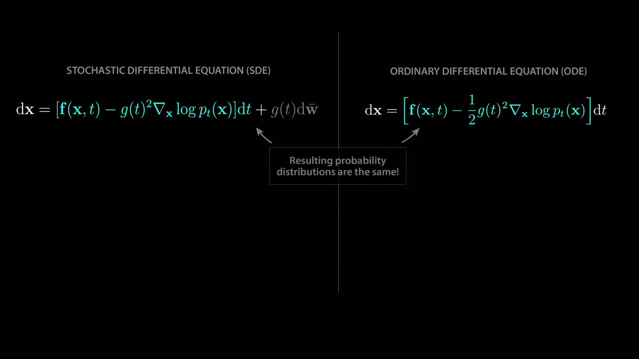
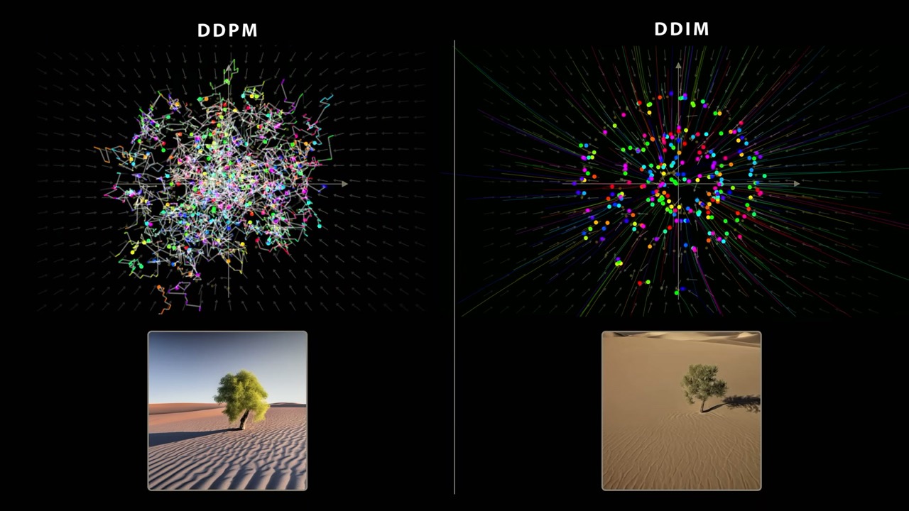
Two equations side by side: a stochastic differential equation with a g(t)dw noise term and an ordinary differential equation with a halved score term and no noise, with a note 'Resulting probability distributions are the same!' — 23:01 — SDE versus ODE. Same learned vector field, same final distribution, no randomness in the ODE. Note it is the distribution that matches, not each individual image.

DDPM and DDIM side by side: DDPM trajectories wander chaotically, DDIM trajectories follow smooth paths to the spiral; both produce a desert tree image below — 24:45 — DDPM (random, many steps) versus DDIM (deterministic, fewer steps) on the same trained model. The step-size schedule is what lets DDIM avoid the blurry-average trap.

DDIM needs no retraining. Wan uses a generalisation of it called flow matching (24:57).

24:57 – 28:16 Steering with text: conditioning

CLIP maps text to vectors but cannot generate; diffusion generates but needs direction. OpenAI combined them in 2022: a diffusion model trained to invert CLIP’s image encoder, called unCLIP and better known as DALL-E 2 (26:14).

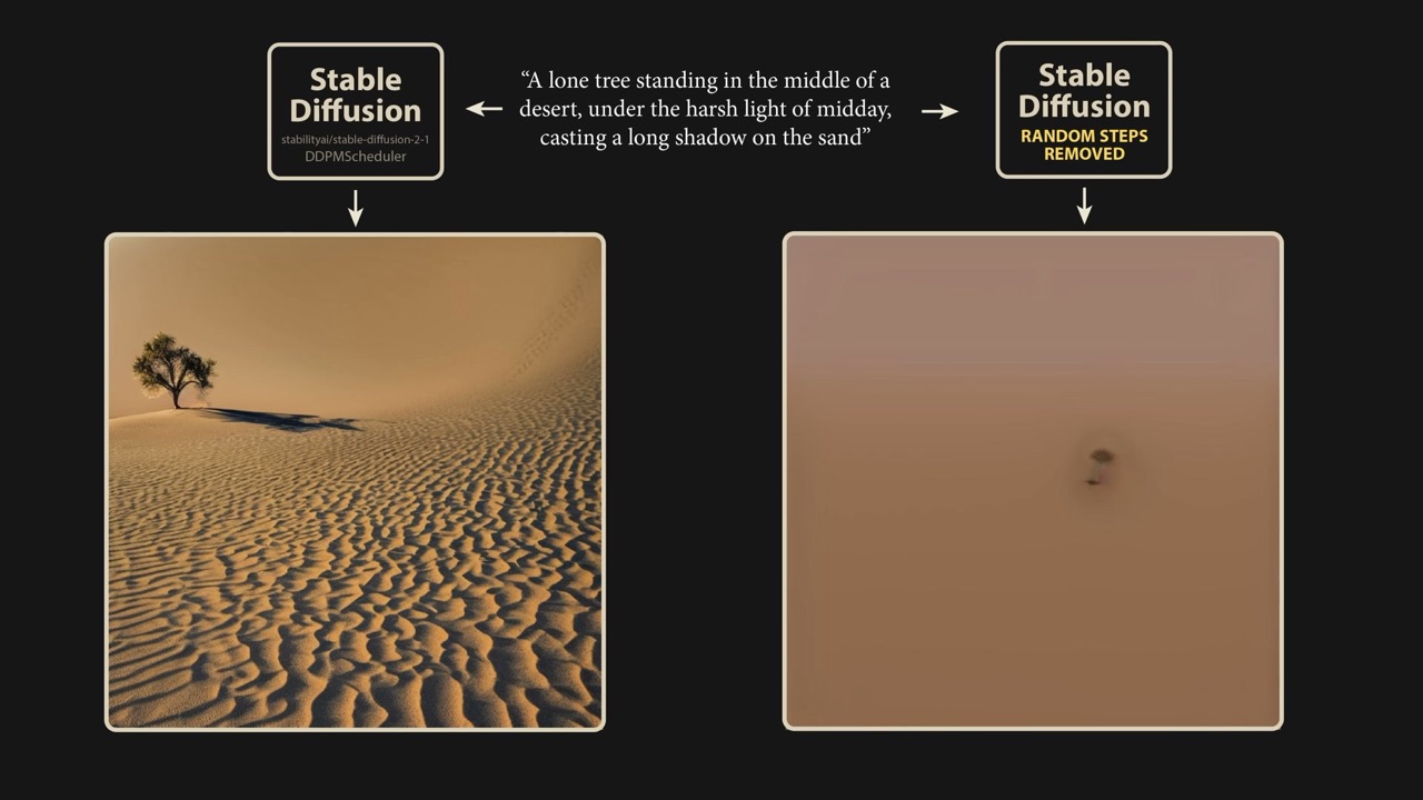
The simplest way to use the text vector is conditioning: feed it to the denoiser as an extra input, just as t was. Methods differ: cross-attention (see the attention chapter), adding or appending the vector, or several at once. But conditioning alone is weak. Stable Diffusion with conditioning only gives a desert and a shadow but no tree (27:59).

28:16 – 34:30 Classifier-free guidance

Back to the spiral, now split into people, dogs and cats. A class-conditioned model recovers the overall shape but fits poorly, because “go toward realistic data” overpowers “go toward cats”.

The fix is to train the same model sometimes without the label, so it can output both an unconditional field and a conditional one. Far from the data they agree; near the data they diverge. Subtract the unconditional vector from the conditional one to isolate “the cat-specific direction”, multiply by α, and step along that (31:08). Points then land neatly on their class’s part of the spiral.

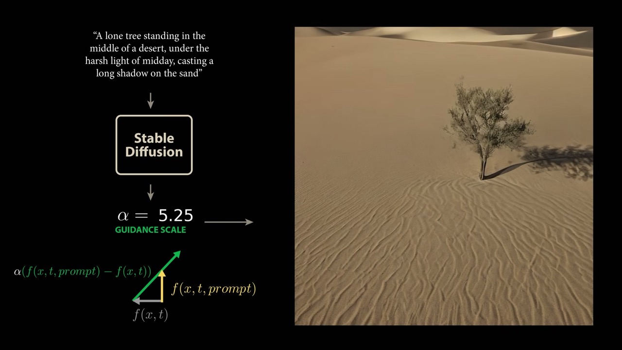
Stable Diffusion with guidance scale alpha = 5.25 producing a detailed tree in a desert, next to a vector diagram of α(f(x,t,prompt) − f(x,t)) — 33:28 — Guidance in practice. At α around 2 a small tree appears; at 5.25 it is large and detailed. The small diagram shows the guided step: conditional minus unconditional, scaled up.

Wan goes one step further with a negative prompt: instead of the empty prompt it subtracts the output for a written list of unwanted features, such as extra fingers or walking backwards, and that negative prompt is written in Chinese. Without it, the astronaut video turns cartoonish (33:37).

34:30 – 37:00 Wrap-up and the guest-video context

Welch’s closing point is that a text encoder trained separately can steer a complex diffusion process at all, and that simple geometric intuitions about vectors hold up in such high dimensions. Grant then explains that this is a guest video by Stephen Welch, commissioned while he was on paternity leave, and recommends the Welch Labs channel (35:01).

Skip list

0:50 – 1:20 Prompt variations on the astronaut demo. Fun, no new ideas.
3:31 – 4:02 Scaling-laws context from 2020 language models.
11:24 – 11:39 Pointer to an external DDPM tutorial.
35:37 – end Grant’s recommendation of Welch Labs and plans for the other guest videos.

Glossary

Diffusion model — a generator that turns noise into data by repeatedly following a learned direction field.
CLIP — paired text and image encoders trained contrastively into one 512-dimensional space.
Cosine similarity — the cosine of the angle between two vectors; 1 means same direction.
DDPM — the 2020 diffusion method that predicts total noise and adds noise at each sampling step.
Score function — the vector field pointing toward more likely, less noisy data.
DDIM — a deterministic sampler, from an equivalent ODE, that needs fewer steps.
Conditioning — giving the model extra input, like time or a text vector.
Classifier-free guidance — stepping along α × (conditional − unconditional output) to strengthen a prompt.

FAQ

Who presents "But how do AI images and videos actually work?" on 3Blue1Brown?

It is a guest video by Stephen Welch, who runs the Welch Labs channel. Grant Sanderson explains at the end that he commissioned a few guest videos while on paternity leave.

How do diffusion models generate images?

They start from pure random noise and repeatedly pass it through a trained network that points toward more realistic data, moving the image a little each step. The video shows this for the open-source Wan 2.1 video model over 50 steps.

Why does DDPM add random noise while generating images?

The model learns to predict the average of where a noisy point came from. Without added noise, every sample drifts toward that average, which in image space looks blurry. Adding noise turns the prediction into a sample from the distribution instead.

What is classifier-free guidance?

The model is run with and without the prompt. The difference between the two outputs points toward what the prompt adds, and it is scaled up by a factor alpha before stepping. This greatly improves how closely images follow the prompt.

Studying another course? Paste its YouTube or Bilibili link on the home page to request a handout — or make your own with the desktop app (coming soon).