3Blue1Brown neural networks ch. 4: backpropagation calculus — notes
Watch the video (10 min)
Watch the original video on YouTube
Chapter 4 turns the intuitive walkthrough of chapter 3 into formulas. It starts with a toy network that has one neuron per layer, uses the chain rule to get the cost’s sensitivity to one weight, then adds indices for full layers. The video assumes you watched chapter 3 and are comfortable with derivatives and the chain rule. It is the most formula-dense video in the series and the one that best repays pausing. Optional for viewers who only want the intuition; essential if you plan to implement backprop yourself.
Key takeaways
- Name the weighted sum z. Then each weight affects the cost through a chain: w → z → a → C (1:38).
- ∂C/∂w is a product of three local derivatives: a(L−1), σ′(z(L)) and 2(a(L) − y) (4:03).
- The bias formula is almost the same, with ∂z/∂b = 1 in place of a(L−1) (5:11).
- ∂z/∂a(L−1) = w(L) is what makes it backpropagation. It hands the sensitivity to the previous layer so the same step can repeat (5:11).
- With many neurons, an earlier activation’s derivative is a sum over paths. Everything else is extra indices (8:28).
Chapter notes
0:00 – 0:34 Goal: how ML people think about the chain rule
Grant states the aim: show how the chain rule is used in networks, which “has a different feel” from a typical calculus course. The difference is that in networks you track sensitivities flowing through a graph of simple operations, rather than differentiating one big closed-form expression.
0:34 – 1:38 The one-neuron-per-layer network
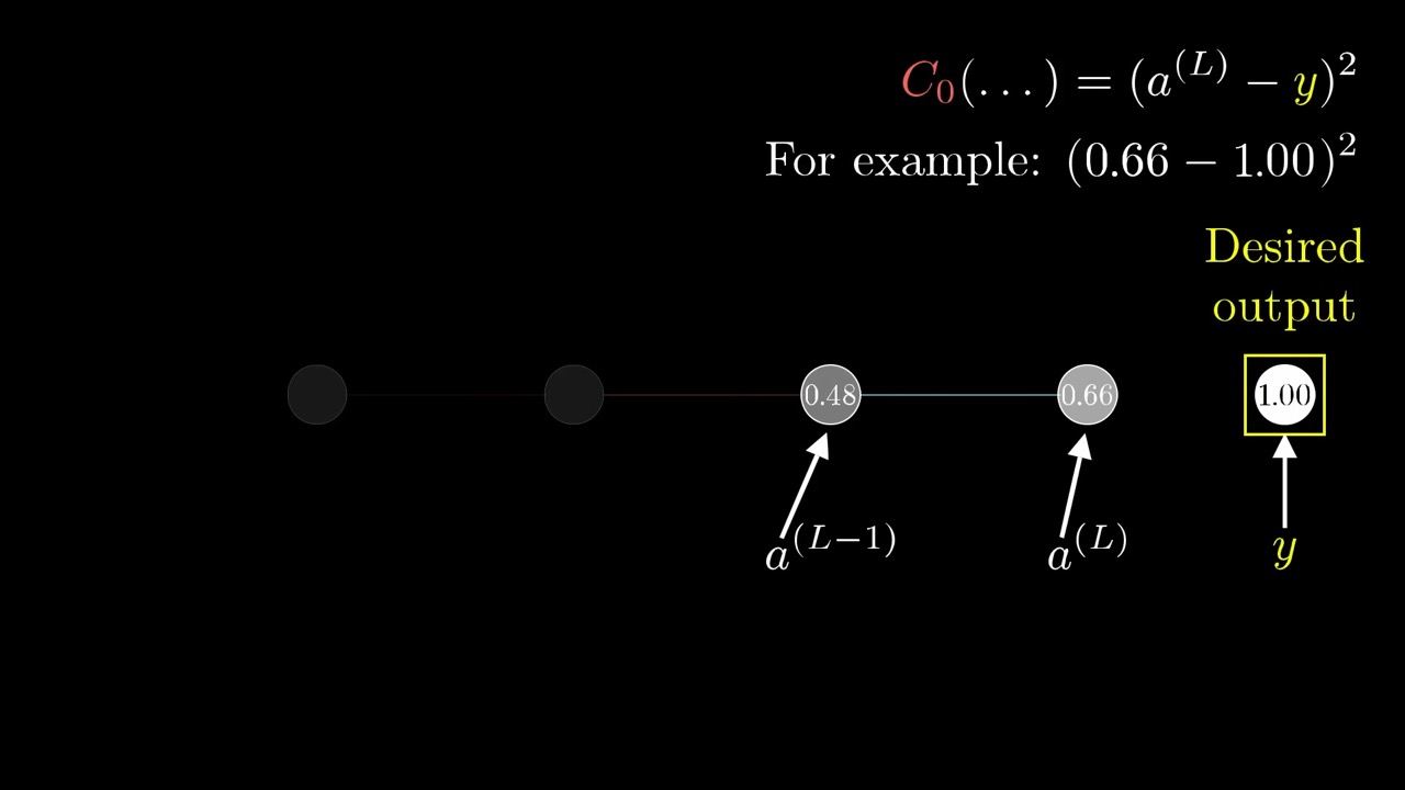
The simplest possible case: four neurons in a row, three weights, three biases. Focus on the last link. Call the last activation a(L) and the one before it a(L−1). The superscripts index layers; they are not powers. For a target y, the cost of one example is C₀ = (a(L) − y)².
1:38 – 3:44 Naming z and drawing the dependency chain
The last activation is a(L) = σ(w(L)·a(L−1) + b(L)). Grant names the inside z(L) = w(L)·a(L−1) + b(L). This one step makes the rest readable. Now the dependencies form a small tree: w, a(L−1) and b feed z; z feeds a; a and y feed C.
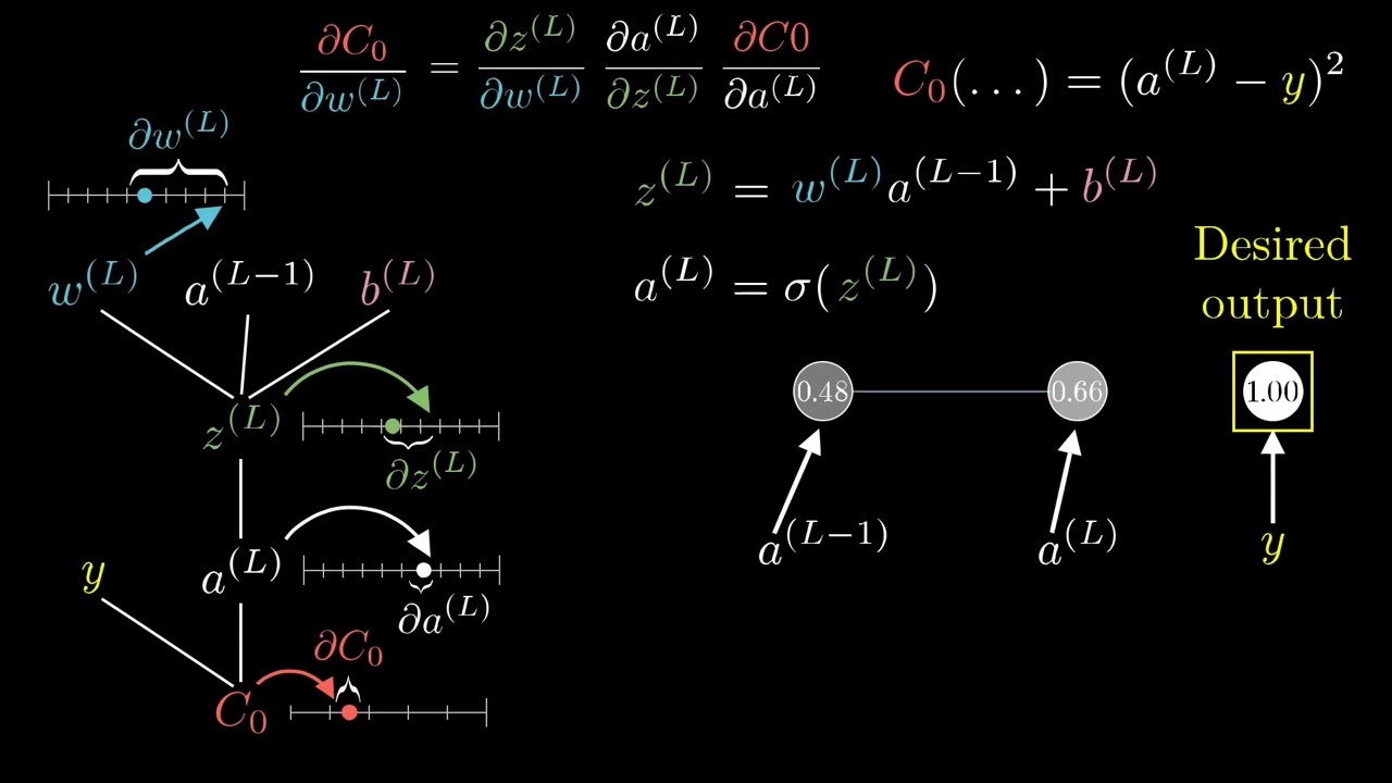
The number-line picture is the best part of the video. Read ∂w as “a tiny nudge, like 0.01” and ∂C as “the resulting nudge to the cost.” Then the chain rule is just the claim that ratios multiply along the chain. It is the same “desired nudge” language as chapter 3, now made exact.
3:44 – 4:49 Computing each factor
Each of the three factors is easy on its own:
- ∂C₀/∂a(L) = 2(a(L) − y). It is large when the output is far from the target, so badly wrong outputs drive the biggest updates.
- ∂a(L)/∂z(L) = σ′(z(L)), the slope of the nonlinearity at the current input.
- ∂z(L)/∂w(L) = a(L−1), the previous activation.
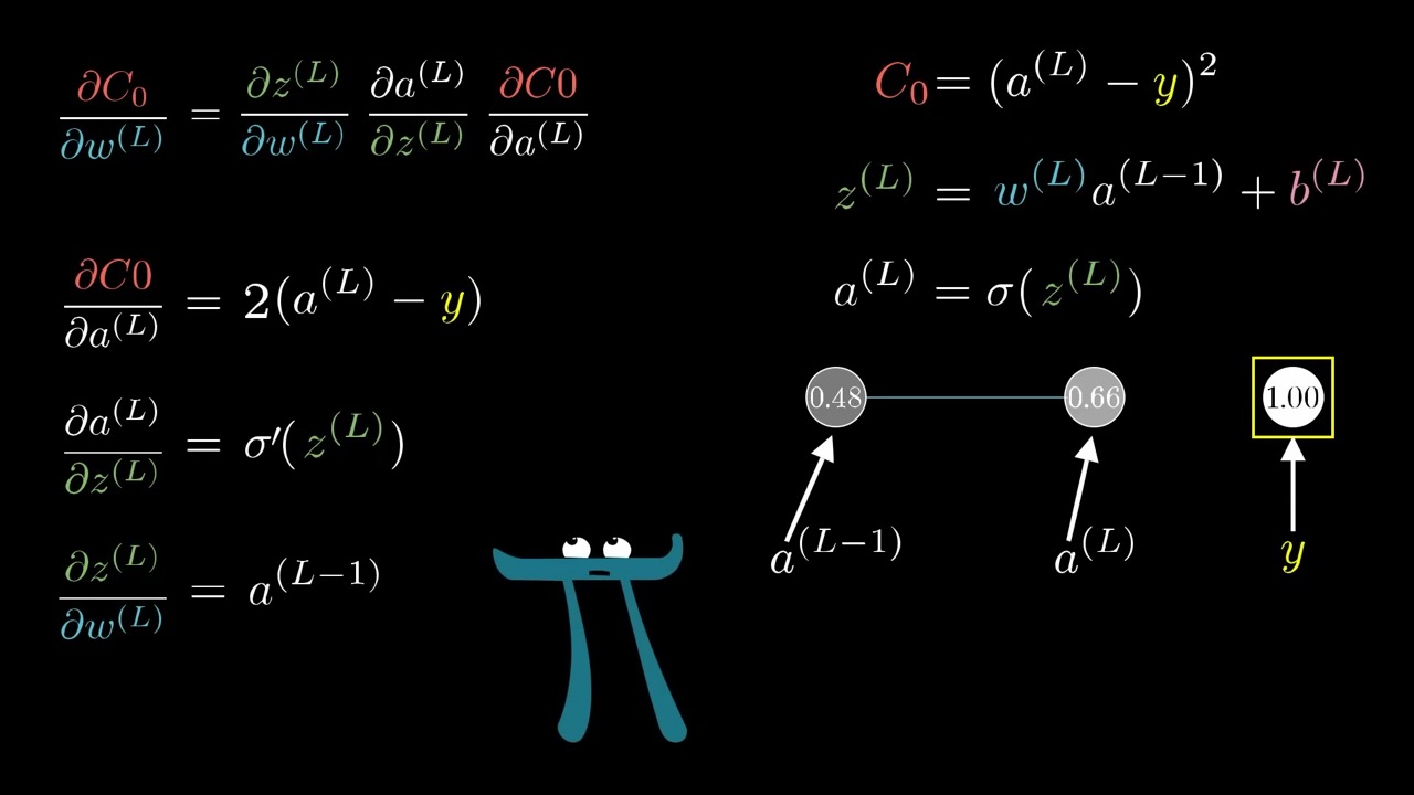
Grant asks you to stop and interpret the last factor. A weight’s influence scales with how active the previous neuron is, which is “fire together, wire together” from chapter 3 written as math.
4:49 – 6:43 Assembling, then bias and previous activation
Multiplying gives ∂C₀/∂w(L) = a(L−1) · σ′(z(L)) · 2(a(L) − y). That covers one example only. The full cost averages over all examples, so its derivative averages this expression. And it is just one of the 13,002 entries of the gradient.
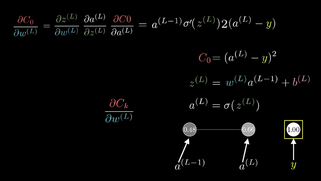
Two variants follow with almost no extra work. For the bias, swap ∂z/∂w for ∂z/∂b, which is 1. For the previous activation, swap in ∂z/∂a(L−1) = w(L). That last one is the hinge of the whole algorithm. You cannot change a(L−1) directly, but knowing ∂C/∂a(L−1) lets you treat layer L−1 as if it were the output and repeat the same three-factor step for w(L−1) and b(L−1).
A practical pitfall: the factor σ′(z) appears once per layer. With a sigmoid, σ′ is at most 0.25 and near zero when the neuron is saturated. Multiply several of these and gradients for early layers shrink. This is one concrete reason chapter 1’s closing interview favors ReLU.
6:43 – 8:28 Many neurons per layer
Real layers have many neurons, so add subscripts. Let k index neurons in layer L−1 and j index neurons in layer L. The cost becomes a sum over outputs: C₀ = Σⱼ (aⱼ(L) − yⱼ)².
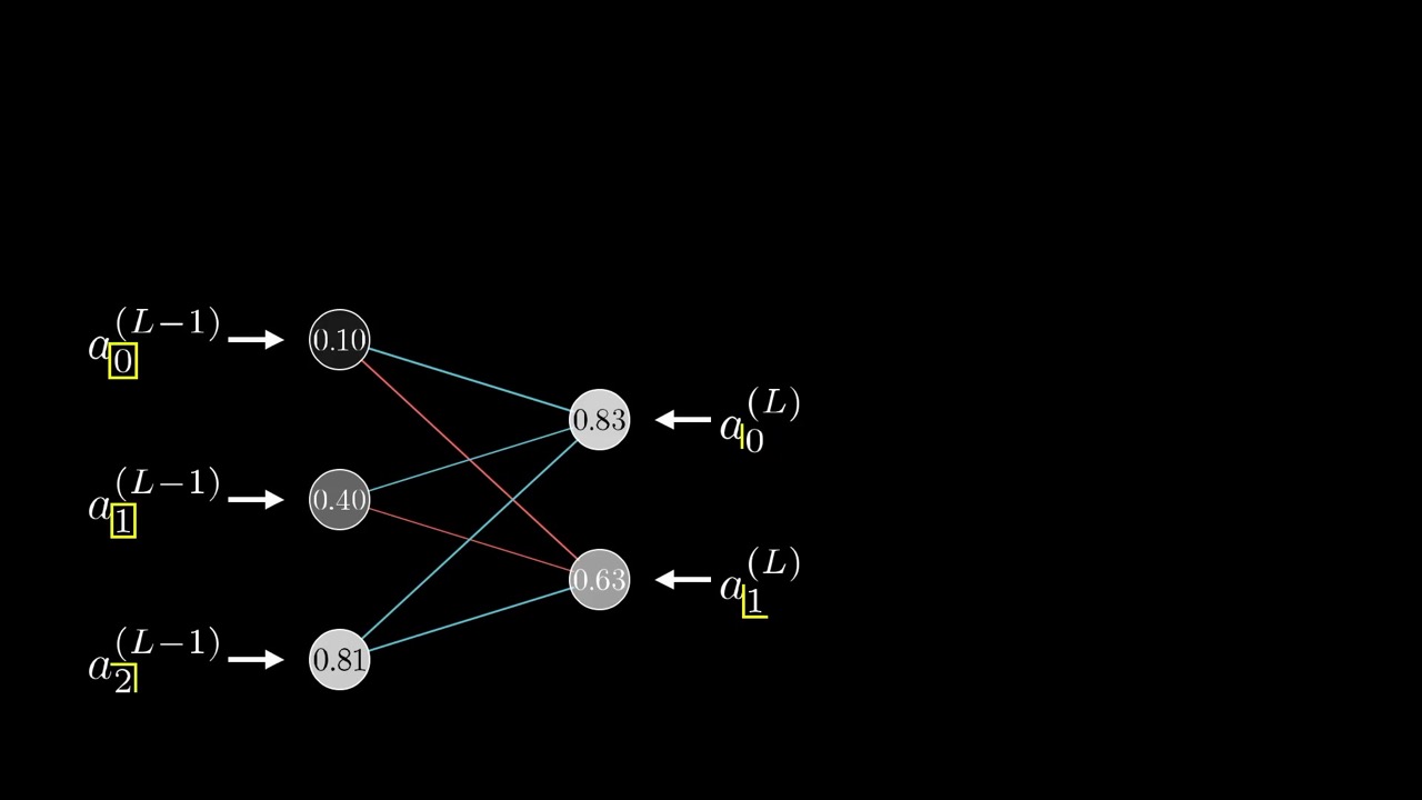
The weight from neuron k to neuron j is wjk(L). The order looks backwards, target first, but it matches the weight matrix from chapter 1, where row j holds the weights into neuron j. With z and a defined per neuron, the derivative for one weight has the same three-factor shape as before.
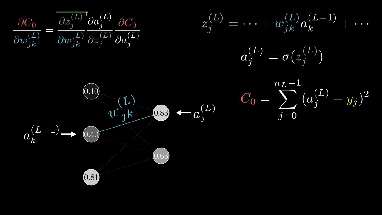
8:28 – 9:24 The one real change: summing over paths
What does change is the derivative with respect to an earlier activation. Neuron k in layer L−1 feeds every neuron in layer L, and each of those affects the cost. So its influence is the sum of the chain-rule products along each path.
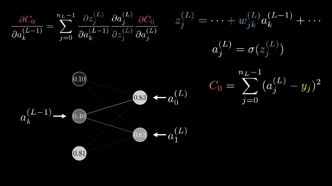
This sum is the precise form of the averaging-of-wishes step at 7:35 in chapter 3. With it, you know ∂C/∂a for every neuron in layer L−1 and can repeat the process all the way to the input.
9:24 – 10:17 The full recipe in one box
The closing slide packs everything into two lines.
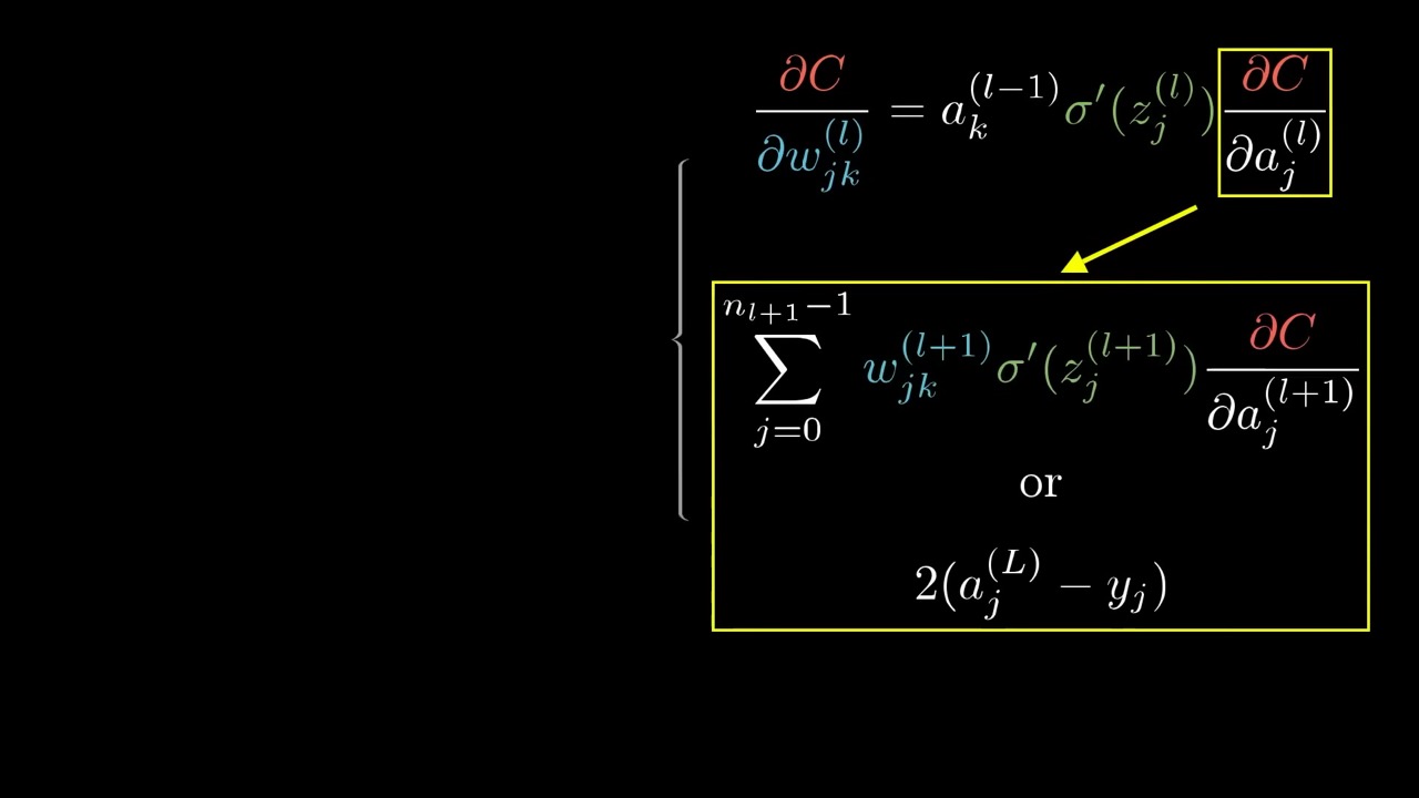
A reading tip for this slide: inside the sum, j runs over neurons in layer l+1, so it is a different j from the one on the left. Read it as “sum over every neuron in the next layer that this neuron feeds.” Libraries vectorize the same recipe with matrices: the sum over j becomes a multiplication by the transposed weight matrix. Grant ends by acknowledging it is “a lot of layers of complexity” and that it is normal to need time.
Skip list
- 0:17 – 0:34 Pause-and-ponder reminder and the calculus series plug.
- 6:43 – 7:03 The “isn’t this oversimplified?” setup. The answer arrives right after.
- 9:37 – 10:17 Closing reassurance and Patreon credits.
Glossary
- Chain rule — the derivative of a composition is the product of the derivatives of each step.
- z (weighted sum) — w·a + b before the nonlinearity; naming it splits the chain into simple pieces.
- σ′(z) — the slope of the activation function at the neuron’s current input.
- Partial derivative ∂C/∂w — how much the cost changes per tiny change in one parameter, holding the rest fixed.
- wjk — the weight from neuron k in the earlier layer to neuron j in the later layer.
- Computational graph — the diagram of which quantities feed which; backprop walks it in reverse.
- Vanishing gradient — the shrinking of early-layer gradients when many small σ′ factors multiply together.
FAQ
What is the formula for the derivative of the cost with respect to a weight?
For a single training example, ∂C/∂w = a(L−1) · σ′(z(L)) · 2(a(L) − y) in the one-neuron case. It is the product of three chain-rule factors: how z depends on w, how a depends on z, and how the cost depends on a.
How does backpropagation use the chain rule?
Each weight affects the cost through a chain: weight to weighted sum z, z to activation a, a to cost. Multiplying the local derivatives along that chain gives the weight's sensitivity, and the derivative with respect to an earlier activation lets you repeat the same step one layer back.
What changes when layers have more than one neuron?
Mostly the indices: weights become w_jk, linking neuron k in layer L−1 to neuron j in layer L. The one real change is that an earlier activation affects the cost through several neurons in the next layer, so its derivative is a sum over those paths.
What is the derivative with respect to the bias?
It is the same chain as for the weight, except ∂z/∂b = 1 replaces ∂z/∂w = a(L−1). So ∂C/∂b = σ′(z(L)) · 2(a(L) − y) for one example in the simple network.
Studying another course? Paste its YouTube or Bilibili link on the home page to request a handout — or make your own with the desktop app (coming soon).