3Blue1Brown neural networks: what is cross-entropy? — notes

Updated 2026-10-02 · Video: 3Blue1Brown, published 2026-07-16 · 34 min

10 key slides

Watch the video (34 min)

Watch the original video on YouTube

This 3Blue1Brown video is Part 2 of a mini-series called “Compression is Intelligence”, and it sits in the neural networks playlist because it explains the loss function used to pre-train language models. The first half builds cross-entropy from compression; the second half shows the same formula appearing in language model training and distillation, and ends with KL divergence. It assumes you know what a language model outputs (see LLMs explained briefly or transformers) and the idea of minimising a loss with gradient descent. It also picks up the robot example and the −log₂ idea from Part 1 of the mini-series; the notes below recap what you need.

Key takeaways

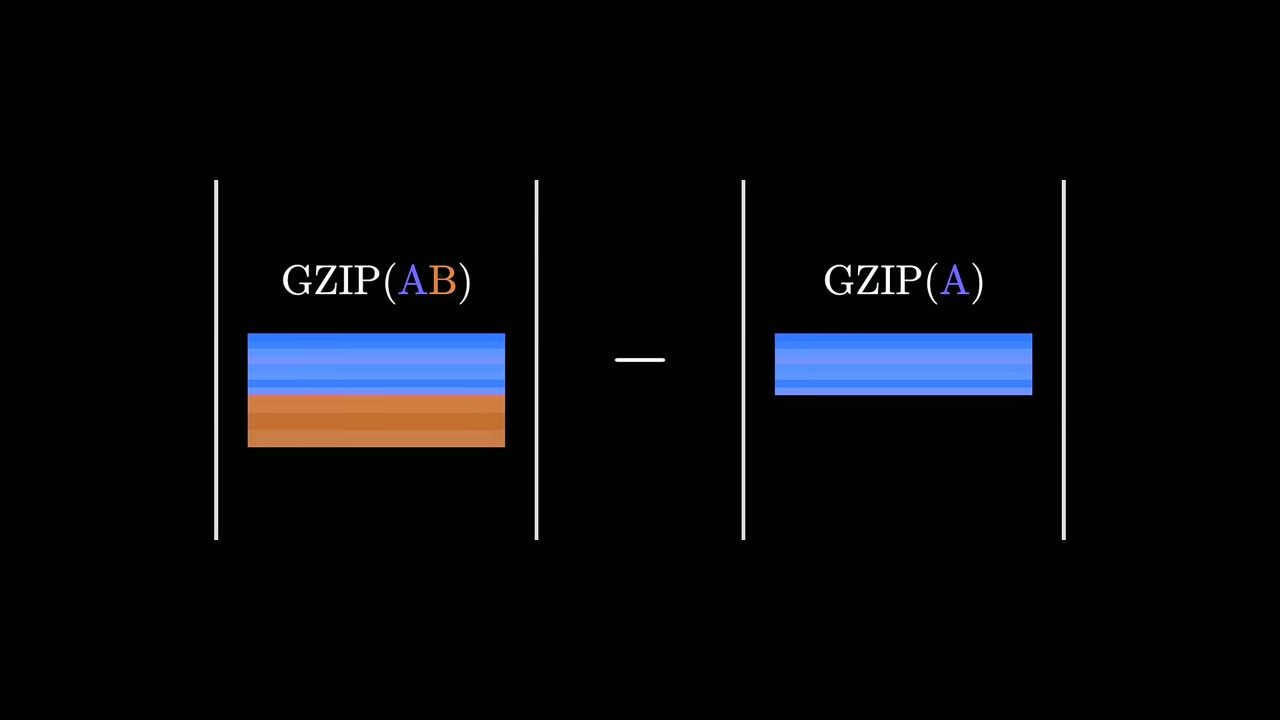
Gzip alone can cluster languages. Compressing document A with a snippet of B appended, versus A alone, measures how different B is from A (0:53).
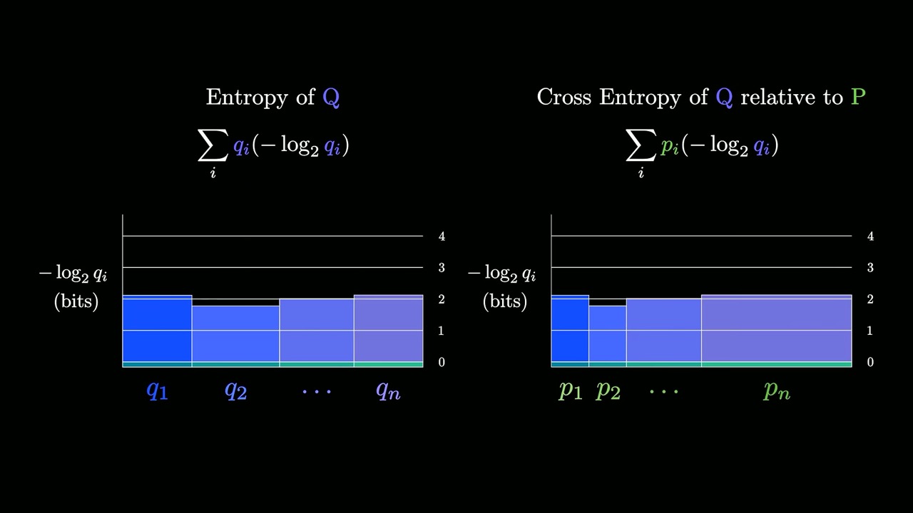
Cross-entropy is the cost of using the wrong code: Σ pᵢ(−log₂ qᵢ), bits per symbol when data follows P but the code was built for Q (6:37).
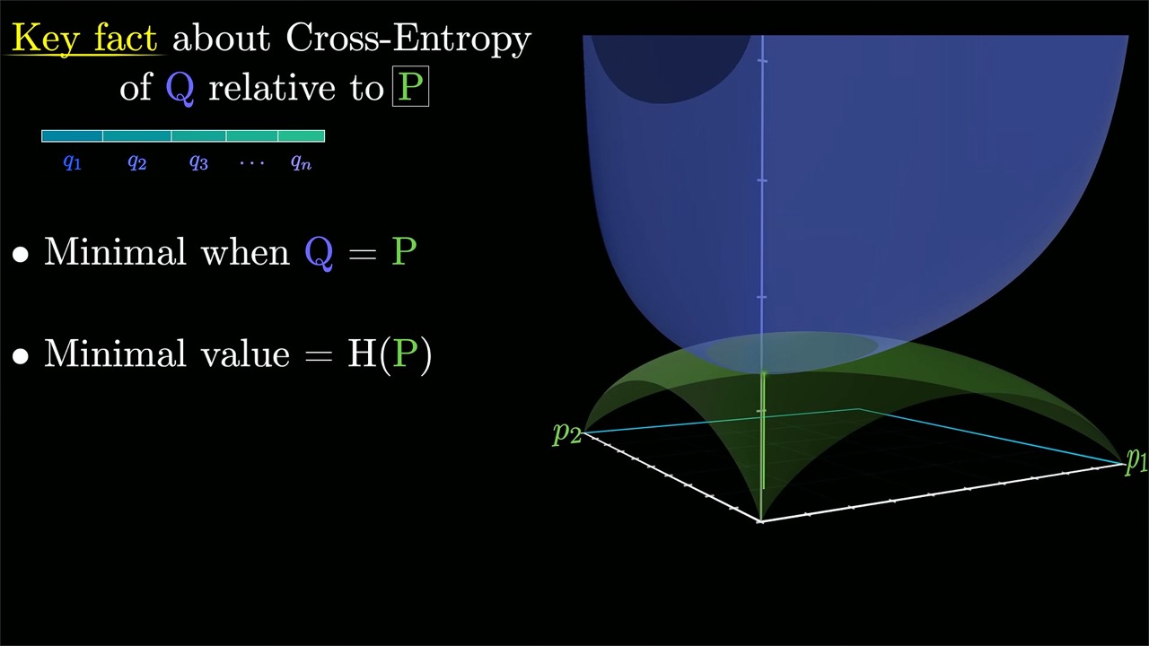
The one fact to remember: with P fixed, cross-entropy is minimal when Q = P, and the minimum is the entropy of P (12:26).
Pre-training loss is average information per token from the model’s view, and grouping identical contexts turns it into cross-entropy against the data’s statistics (17:35).
Distillation uses cross-entropy against a teacher’s full distribution, a much richer signal than one true token (26:58).
KL divergence is cross-entropy minus entropy, the bits wasted by a mismatched code (31:56).

Chapter notes

0:09 – 3:03 Language trees and zipping

The video opens with a 2002 paper, “Language Trees and Zipping”, that recovered relationships between languages using only general-purpose file compression. The trick: append a small piece of document B to document A, compress, and compare with compressing A alone.

Two bars: GZIP(AB), with a blue part for A and an orange part for B, minus GZIP(A), a blue bar — 1:04 — The co-compression distance. The orange extra is small when B resembles A, because the compressor has already "learned" A's patterns. Hold on to this picture; it is cross-entropy in disguise.

The plan of the video is laid out next: first cross-entropy from compression, then pre-training and distillation, then a reframing of LLM training as compression (2:48).

3:03 – 6:37 Information and the robot code

Recap from Part 1: you send a stream of four robot instructions with probabilities ½ (up), ¼ (down), ⅛ (left), ⅛ (right). The best code spends 1, 2, 3 and 3 bits on them. In general an optimal code spends about −log₂ p bits on a symbol of probability p. Claude Shannon called that the information content. It does not have to be a whole number: a long message costs about the sum of its symbols’ information.

Now the space agency rotates the plan so right is most common (½), left ¼, up and down ⅛ each, but the old code stays hard-wired.

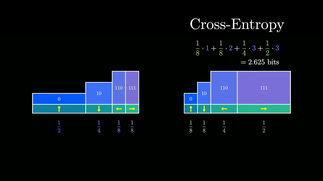
Two bar diagrams of the robot codes 0, 10, 110, 111; on the right the widths follow the new probabilities 1/8, 1/8, 1/4, 1/2 and the sum 1/8·1 + 1/8·2 + 1/4·3 + 1/2·3 = 2.625 bits — 6:37 — The old code under the new reality costs 2.625 bits per instruction. Bar width is how often a symbol appears (new P), bar height is its code length (old Q). Area is the cross-entropy.

A quick check you can do yourself: the new distribution is the old one shuffled, so a code built for it would cost 1.75 bits. The gap of 0.875 bits is waste, which the video later names KL divergence.

6:37 – 12:50 The formula and its key property

Call the true distribution P and the one the code was built for Q. Entropy of Q is Σ qᵢ(−log₂ qᵢ). Cross-entropy of Q relative to P keeps the heights −log₂ qᵢ but uses the widths pᵢ. Grant notes the notation in the wild is a mess (H(P,Q), H(P‖Q), and others) and sticks to the sum itself (8:11).

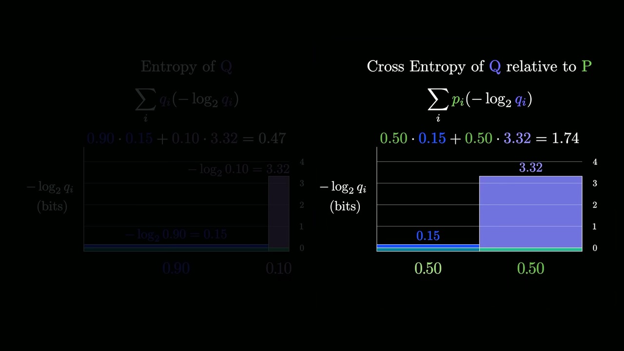
Side by side: 'Entropy of Q' as sum q_i(−log2 q_i) with bars of width q_i, and 'Cross Entropy of Q relative to P' as sum p_i(−log2 q_i) with the same heights but widths p_i — 8:16 — The diagram that makes the formula readable: heights come from Q (the code), widths from P (reality). Switch which distribution sets the widths and you switch between entropy and cross-entropy.

Order matters. If Q is 50/50 and P is 90/10, every symbol costs 1 bit, so cross-entropy is 1 bit. Swap them and the code built for 90/10 spends about 3.32 bits on the symbol it thought was rare, which now appears half the time.

Cross entropy of Q relative to P with Q skewed 0.90/0.10 and P even: 0.50·0.15 + 0.50·3.32 = 1.74, shown as two bars of heights 0.15 and 3.32 and widths 0.50 — 10:04 — The asymmetric case: 1.74 bits, versus 1 bit the other way round. Cross-entropy is not a distance; swapping P and Q changes the value.

With only two outcomes, each distribution has one free number, so Grant can plot cross-entropy against q₁ for a fixed p₁. The curve has a clear minimum exactly where q₁ = p₁. Moving p₁ and tracing the minima draws the entropy curve (11:31).

Slide 'Key fact about Cross-Entropy of Q relative to P: Minimal when Q = P; Minimal value = H(P)' next to a blue bowl-shaped surface touching a green entropy surface — 12:26 — The key fact. Grant asks viewers to remember only this. Every later use of cross-entropy (training, distillation, KL) leans on it.

12:50 – 15:22 Back to zipping

Gzip(AB) − gzip(A) asks the cross-entropy question (13:16): how well does a scheme tuned to A handle B? It is only a rough empirical estimate. It compares samples, not distributions, and gzip, which replaces repeats with pointers to earlier text, is far from the Shannon limit. The authors’ actual metric is a bit more complicated. Still, it was good enough to recover language families, and the general lesson is that cross-entropy measures how different the patterns of two settings are.

15:22 – 20:38 Pre-training loss as average information per token

A language model maps text to a distribution over the next token. Training needs a loss whose minimum means good predictions; gradient descent and backpropagation do the rest. Grant’s description of the standard loss: for every position in the training text, take the probability the model gave to the true next token and compute its −log, then average over all tokens.

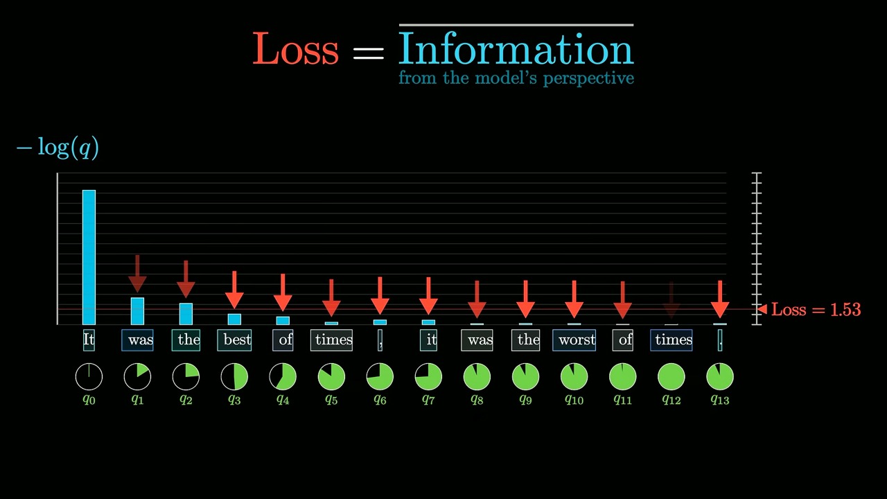
'Loss = Information from the model's perspective': bars of −log(q) above each token of 'It was the best of times, it was the worst of times', shrinking with red arrows, average loss 1.53 — 18:28 — Loss as the model's surprise. A better model gives the true tokens higher probability, so the bars shrink. All these probabilities come out of one forward pass.

In practice natural log replaces log₂; they differ by a constant that the learning rate absorbs, and natural logs give cleaner derivatives (19:07). Batching, optimizers and scale are glossed over on purpose. The open question Grant leaves hanging: many decreasing functions punish low probabilities, so why the log?

20:38 – 25:54 Why it is called cross-entropy, and why the log is forced

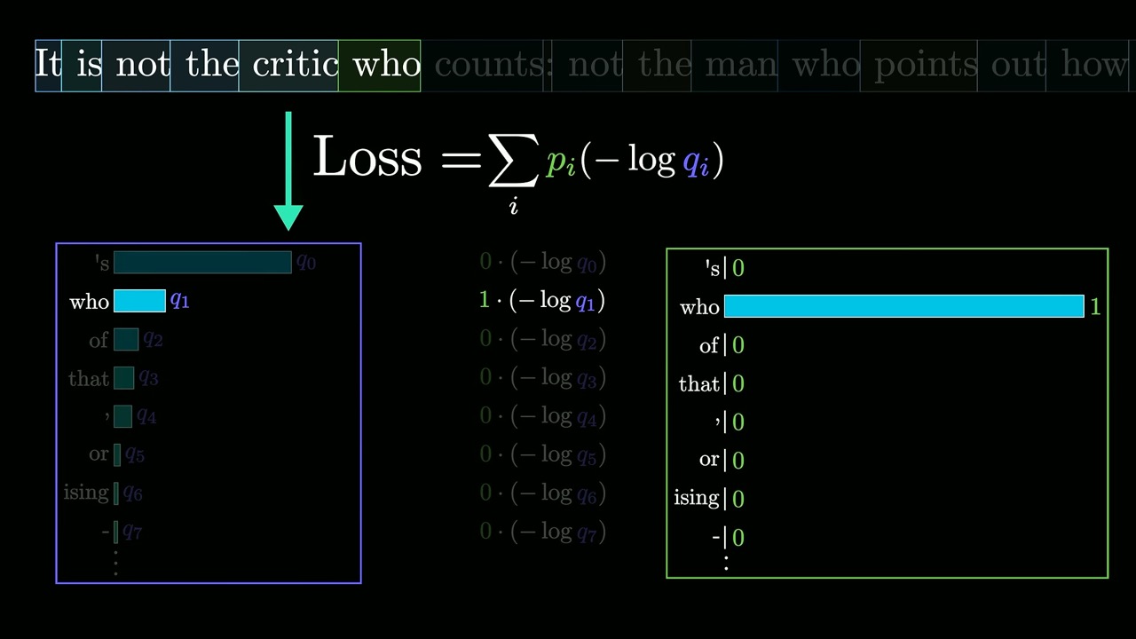
The common explanation is that you compute cross-entropy against a one-hot distribution with all mass on the true token.

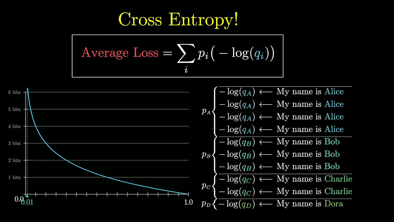
For the text 'It is not the critic who', the model's distribution over next tokens beside a one-hot distribution with 1 on 'who', and the sum p_i(−log q_i) collapsing to 1·(−log q_1) — 21:14 — The one-hot story. All the zero weights cancel, leaving −log of the true token's probability. Grant calls this explanation unsatisfying because it does not say why cross-entropy is the right thing to use.

His better explanation groups examples. Take the context “My name is”. In the data, each name appears with some frequency pᵢ; the model gives each name a probability qᵢ. The total loss over all examples with this context is Σ pᵢ·f(qᵢ) for whatever per-example function f you chose. Choose f = −log and that is exactly cross-entropy of the model relative to the data.

'Cross Entropy!' with 'Average Loss = sum p_i(−log(q_i))' boxed, beside the −log curve and a list of training examples 'My name is Alice/Bob/Charlie/Dora' grouped by frequency — 25:54 — Summing per-example losses over a shared context gives weights pᵢ for free. With f = −log, the average loss is the cross-entropy formula, so it is minimised when the model's q matches the data's p.

The argument also runs backwards. If you demand that the average loss be minimised only when q = p, a Lagrange multiplier argument forces f′(q) to be a constant over q, and only logarithms do that (25:05). The details are on screen for those who want to pause. The practical upshot: the log in the loss is not a stylistic choice.

26:13 – 28:05 Distillation

To make a small model behave like a large one, run both on the same text. At each position compare the small model’s full distribution with the large model’s full distribution, using cross-entropy, instead of with the single true token.

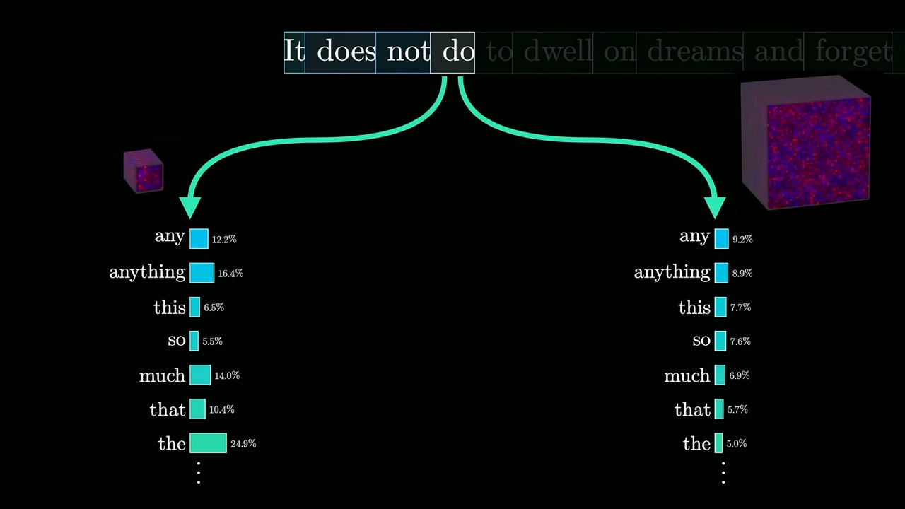
The text 'It does not do' branching to a small model and a large model, each showing a probability distribution over next tokens such as any, anything, this, so, much, that, the — 26:58 — Distillation: the small model's target is the big model's whole distribution. Grant compares it to learning chess from a strong player who talks through every good move, instead of just watching one game.

This connects to the “My name is” example: with a teacher, a single example already carries a full distribution over names, instead of needing thousands of examples to build it up.

28:05 – 30:01 Wrap-up and the compression teaser

Cross-entropy arose naturally from compression in the first half (28:17); in the second half it came from constrained optimisation. Grant argues the two are connected and promises Part 3: a compression algorithm that turns any predictor into a compressor whose output length matches the model’s information content. That would make cross-entropy training the same as training the best possible text compressor.

31:38 – 33:30 KL divergence

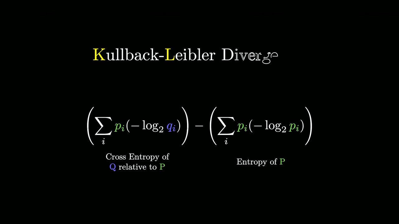
'Kullback-Leibler Divergence' written as (sum p_i(−log2 q_i)) − (sum p_i(−log2 p_i)), labelled cross entropy of Q relative to P minus entropy of P — 31:56 — KL divergence is cross-entropy minus entropy: the bits per symbol wasted by the wrong code. For the robot example it is 2.625 − 1.75 = 0.875 bits.

KL divergence acts like a distance between distributions, zero when they match, but it is asymmetric. Grant leaves three exercises: show the compact single-sum form equals the difference, read the KL version of the bar diagram, and think about what changes if distillation used KL instead of cross-entropy. (Hint for the last one: the teacher’s entropy does not depend on the student, so it does not change the gradients.)

Skip list

2:14 – 3:03 Outline of the video.
3:03 – 5:01 Recap of Part 1. Skip if you know information as −log₂ p; our notes above cover it.
20:09 – 20:38 List of engineering details (batching, optimizers) that the video explicitly sets aside.
30:01 – 31:38 Plug for 3Blue1Brown’s virtual career fair and a partner company’s challenge.

Glossary

Information content — −log₂ p, the bits an optimal code spends on an event of probability p.
Entropy H(P) — the average information of a distribution; the best possible bits per symbol.
Cross-entropy — Σ pᵢ(−log qᵢ), the average cost when data follows P but the code or model follows Q.
Cross-entropy loss — the average −log probability a model gives to the true next token.
One-hot distribution — all probability on a single outcome.
Distillation — training a small model on a larger model’s output distributions.
KL divergence — cross-entropy minus entropy; the waste from a mismatched distribution.

FAQ

What is cross-entropy in simple terms?

It is the average number of bits per symbol you spend when you encode data from one distribution, P, using a code optimised for another distribution, Q. The formula is the sum of p_i times −log q_i.

Why is cross-entropy minimised when the two distributions match?

A code built for the true distribution is the most efficient one possible. With P fixed, cross-entropy is smallest exactly when Q equals P, and that smallest value is the entropy of P.

Why is language model loss called cross-entropy loss?

Averaging −log of the probability the model gives each true next token, over all examples sharing a context, is exactly the cross-entropy of the model's distribution relative to the data's. The video also argues that if you want the loss minimised only when the model matches the data, the function must be a logarithm.

What is KL divergence?

It is cross-entropy minus entropy: the extra bits per symbol you waste by using a code built for the wrong distribution. It is zero when the distributions match and is not symmetric.

Studying another course? Paste its YouTube or Bilibili link on the home page to request a handout — or make your own with the desktop app (coming soon).